Broadcasting magic ✨

import torch
import matplotlib
import matplotlib.pyplot as plt
import torch.nn.functional as F

An important aspect of writing efficient Deep Learning code is to understand the basic operations one can do with tensors. Those include math operations like addition and multiplication or methods like view and transpose. Check out https://fleuret.org/ee559/ee559-slides-1-5-high-dimension-tensors.pdf to have a visual understanding of how these operations work. Another important concept is the so-called “broadcasting” mechanism, which automatically expands dimensions of size 1 when shapes of tensors don’t match.

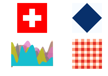
Let’s learn this concept by drawing some figures using only PyTorch tensor operations! By the end of this tutorial, you will know how to draw a picnic tablecloth, a rotated square or even a Swiss flag in PyTorch.

1. Picnic tablecloth

Instead of a boring checkerboard, let us start with a picnic tablecloth pattern.

Constraint: the only raw PyTorch ingredient you’re allowed to use and operate on is torch.arange(2), i.e. a [0, 1] tensor.

x = torch.arange(2); x

Solution to problem 1

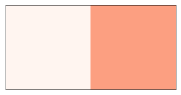
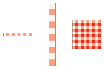
Let us first visualize our tensor. A neat trick is to unsqueeze the first dimension (i.e. add a dimension of size 1), so that our tensor becomes a 2D matrix (of shape [1, 2]). Don’t hesitate to check the shapes of tensors at any point in this tutorial by typing *.shape. Doing this helps a lot in understanding what’s going on.

plt.imshow(x.unsqueeze(0), cmap="Reds", vmin=0, vmax=3)

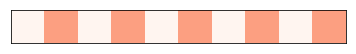
By using the repeat operator, we can repeat the 0-1 pattern as many times as we want.

y = torch.arange(2).repeat(5)

plt.imshow(y.unsqueeze(0), cmap="Reds", vmin=0, vmax=3)

Let us draw our pattern vertically now. This is easily done by inserting a new dimension at the second dim (instead of the first one). We now have a 2D matrix of shape [10, 1].

plt.imshow(y.unsqueeze(1), cmap="Reds", vmin=0, vmax=3)

In order to create our picnic tablecloth, what we’d like to do is to pull those flat shapes towards the bottom and the right (respectively). We could do that by using again the repeat operator and then summing.

z1 = y.unsqueeze(0).repeat(10, 1)
z2 = y.unsqueeze(1).repeat(1, 10)
s = z1 + z2

plt.subplot(1, 3, 1)
plt.imshow(z1, cmap="Reds", vmin=0, vmax=3)

plt.subplot(1, 3, 2)
plt.imshow(z2, cmap="Reds", vmin=0, vmax=3)

plt.subplot(1, 3, 3)
plt.imshow(s, cmap="Reds", vmin=0, vmax=3)

Using the “broadcasting” mechanism, the repeat operation can be handled implictely by PyTorch, by just summing two matrices of shape [1, 10] and [10, 1]. Thus, discarding repeat in the previous code leads to the exact same result (the repeat operations just happen under the hood now). This results in cleaner and faster code. Magic!

z1 = y.unsqueeze(0)
z2 = y.unsqueeze(1)
s = z1 + z2

plt.subplot(1, 3, 1)
plt.imshow(z1, cmap="Reds", vmin=0, vmax=3)

plt.subplot(1, 3, 2)
plt.imshow(z2, cmap="Reds", vmin=0, vmax=3)

plt.subplot(1, 3, 3)
plt.imshow(s, cmap="Reds", vmin=0, vmax=3)

plt.subplot(1, 3, 3)
plt.imshow(s, cmap="Reds", vmin=0, vmax=3)

2. Rotated square

If you’ve well understood the mechanisms involved in the first example, we can start working on the slightly more complicated example of the rotated square.

Constraint: all you’re allowed to use is a torch.linspace(0, 1, 10).

Hint: Broadcasting not only works with math operators (e.g. +) but also also with inequalities (e.g. >).

l = torch.linspace(0, 1, 10); l

Solution to problem 2

Again, let us visualize first our 1D array by unsqueezing the first dimension.

plt.imshow(l.unsqueeze(0).repeat(1, 1), cmap="Blues", vmin=0, vmax=1)
plt.xticks([], []); plt.yticks([], []);

We want the values to be symmetrical around the center. This can be done by subtracting 0.5 and applying the absolute value.

x = 1 - (l - .5).abs()

plt.imshow(x.unsqueeze(0).repeat(1, 1), cmap="Blues", vmin=0, vmax=1)

Now let us compare this array to the first value of l:

x.unsqueeze(0) > l[0]

All values of x are larger than l[0] which is 0. Notice that this intuitive operation uses a form of broadcasting under the hood since we compare a 1D tensor to a scalar. We would get the same result if we wrote: x.unsqueeze(0) > torch.tensor(l[0]).repeat(10) where each element of x is compared one-by-one to the right-hand-side. On the contrary, all values of x are smaller than l[-1] (= 1.0).

x.unsqueeze(0) > l[-1]

By comparing x sequentially to all values of l, we get this downwards triangle pattern.

for threshold in l:
    plt.figure()
    plt.imshow(x.unsqueeze(0) > threshold, cmap="Blues", vmin=0, vmax=1)

By comparing x to l-1, we obtain the same shape but upwards.

for i in range(10):
    plt.figure()
    plt.imshow(x.unsqueeze(0) > (1-l)[i], cmap="Blues", vmin=0, vmax=1)

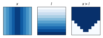
This is where broadcasting comes to the rescue. Instead of writing slow Python for-loops, we can simply compare x.unsqueeze(0) and l.unsqueeze(1).

down_tri = x.unsqueeze(0) > l.unsqueeze(1)
up_tri = x.unsqueeze(0) > (1-l).unsqueeze(1)

plt.imshow(down_tri, cmap="Blues", vmin=0, vmax=1)

To be clear again, doing this expands under the hood the 1D array at the dimension where its size is 1, in order to perform element-wise comparisons.

plt.subplot(1, 3, 1)
plt.imshow(x.unsqueeze(0).repeat(10, 1), cmap="Blues", vmin=0, vmax=1)
plt.title("$x$")

plt.subplot(1, 3, 2)
plt.imshow(l.unsqueeze(1).repeat(1, 10), cmap="Blues", vmin=0, vmax=1)
plt.title("$l$")

plt.subplot(1, 3, 3)
plt.imshow(down_tri, cmap="Blues", vmin=0, vmax=1)
plt.title("$x > l$");

All what’s remaining now is to perform a logical AND between down_tri and up_tri. For PyTorch tensors, this is done using the & symbol (| for OR).

square = (x[None] > l.unsqueeze(1)) & (x[None] > (1-l).unsqueeze(1))
plt.imshow(square, cmap="Blues", vmin=0, vmax=1)

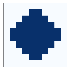
Now, this figure looks a little coarse. By starting with l of size 1000, we obtain a much nicer rotated square in only 3 lines of code!

l = torch.linspace(0, 1, 1000)
x = 1 - (l - .5).abs()
square = (x.unsqueeze(0) > l.unsqueeze(1)) & (x.unsqueeze(0) > (1-l).unsqueeze(1))

plt.imshow(square, cmap="Blues")
plt.axis("off");

Bonus 1: Drawing the Swiss flag

Even though the Swiss flag may not seem very complex, this example is a little more involved if we follow the official proportions of the flag, as described in https://en.wikipedia.org/wiki/Flag_of_Switzerland#Design. Feel free to check the code below and understand what’s happening. However, the basic idea is very easy: we divide an array (of size n) in 5 areas of values 0, 1, 2, 1, 0, reshape it to [1, n] and [n, 1] and perform an addition (making use of the broadcasting mechanism). We then map values above 3 to 1 and the rest to 0. A custom Matplotlib colormap then does the trick.

l = torch.linspace(0, 1, 6+7+6+7+6)
x = ((0.5 - (l - 0.5).abs()) * (6+7+6+7+6)).ceil() // 7

plt.imshow(x.unsqueeze(0).repeat(5, 1), vmin=0, vmax=4)

plt.imshow(x.unsqueeze(0) + x.unsqueeze(1), vmin=0, vmax=4)

l = torch.linspace(0, 1, 6+7+6+7+6)
x = ((0.5 - (l - 0.5).abs()) * (6+7+6+7+6)).ceil() // 7
flag = (x.unsqueeze(0) + x.unsqueeze(1)) > 2

plt.imshow(flag, cmap=matplotlib.colors.ListedColormap([(1, 0, 0), (1,)*3]))
plt.axis("off");

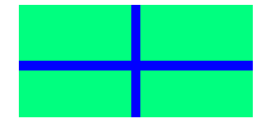
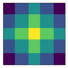
Bonus 2: Drawing a Xmas gift

x = torch.zeros(25, dtype=torch.int)
y = torch.zeros(12, dtype=torch.int)
x[12] = y[6] = 2019
plt.imshow(1 - (x.unsqueeze(0) | y.unsqueeze(1)),
           cmap="winter")
plt.axis("off");