Autogradlib
In this project, I built a small deep learning framework called Autogradlib using only PyTorch’s Tensor operations and the standard math library. The autograd mechanism and the high-level syntax are inspired by PyTorch.
Code is available here: https://github.com/alexandre01/autogradlib.
Autogradlib builds a gradient operations directed acyclic graph (DAG) on the fly, which enables to perform efficiently the backprop algorithm and to draw the associated graph using graphviz (see next figure).
 The gradient operations graph associated to the final network. This graph is rendered automatically in Autogradlib with the
 draw_graph method.
Implementation details
The code structure is shown in figure below.
 Autogradlib’s code structure including the three main classes
 Variable, GradOperator and Module, and some classes that inherit from the latter.
The Variable and GradOperator base classes
Like in PyTorch, when building a neural network, we wrap Tensors in a Variable object. The Variable class stores:
- tensor: the wrapped
Tensor - grad: the gradient of the loss w.r.t. the tensor
- grad_op: the
GradOperatorinstance that actually performs the backpropagation of gradients
The GradOperator class stores:
- variable: the wrapped output variable
- children: the children nodes in the gradient operations DAG
Thus, when running the following piece of code:
x = Variable(FloatTensor(3, 3).normal_())
y = x.t() - x.exp()
z = y.pow(2).sum()
dot = z.draw_graph()
dot.render("model.gv", view=True)
it will produce an underlying tree of GradOperators that we show in the following figure :
 A simple DAG representing the computation
 (x.t() - x.exp()).pow(2).sum()
When we then call z.backward(), the Variable object makes a call to self.grad_op.pass_grad(FloatTensor([1])) which in turn passes recursively the gradient to the GradOperator child nodes.
GradOperator::pass_grad(gradwrtoutput) takes as argument the gradient of the loss w.r.t. the output. The method accumulates the current variable’s grad with this provided gradient and passes to its children the gradient of the loss w.r.t. their respective outputs.
The GradOperator subclasses
The GradOperator subclasses are responsible of:
- computing the output
Variable(in the constructor) - implementing the
pass_grad(self, gradwrtoutput)method to actually perform the backward pass.
I implemented 11 subclasses (see grad package) that enable to perform most of the needed operations in Deep Learning (addition, coefficient-wise multiplication, matrix multiplication, transposition, sum along a specified axis…). To define pass_grad, we use the chain rule. See for instance grad/AddOperator.py which takes as input two Variables $a$ and $b$, stores, the output Variable(a.tensor + b.tensor) and passes the unchanged gradwrtoutput to the two children in the backward pass. Indeed, let $f = a + b$. Then
As another example, see grad/ExpOperator.py. If we define $B = \exp(A)$, where $A$ and $B$ are tensors of same size and $\exp$ is applied coeffient-wise, then we have:
and thus: \(\frac{\partial l}{\partial A} = \exp{A} \odot \frac{\partial l}{\partial B}\)
The Module class
This class is the easiest one to implement. It defines:
- a virtual method
forward(input)that all its subclasses must implement - the method
zero_grad()that re-initializes the gradients of theModule’s parameters params(): automatically computes the list of theModule’s parameters by checking its attributes. The supported parameter types areVariable,ModuleandlistofVariableorModule
Once the Module class is implemented, defining subclasses like ReLU or Sigmoid simply consists of overriding the forward(self, x) method, generally in one line of code! (parameters are computed automatically by Module and the backward pass is handled by the corresponding Variable).
The more tricky part was Softmax since it required to implement two new Variable methods: sum along a specified dimension and repeat in order to multiply two similar sized tensors (since I didn’t implement broadcasting like in PyTorch).
Finally, in order to deal with the vanishing gradients problem and control the variance of both activations and gradients of the loss w.r.t. the activations, we have to make sure to initialize the weights using e.g. Xavier initialization (see implementation in the Linear class).
Results
Evaluation
We train a network with two input units, two output units and three hidden layers of 25 units.
Sequential(
  0: Linear(in_dim=2, out_dim=25)
  1: ReLU
  2: Linear(in_dim=25, out_dim=25)
  3: ReLU
  4: Linear(in_dim=25, out_dim=25)
  5: ReLU
  6: Linear(in_dim=25, out_dim=2)
  7: Softmax(dim=1)
)
Training this model during 500 epochs (repeated 20 times to also compute the variance) gives the following results:
| Loss (median ± std.) | Accuracy (median ± std.) | |
|---|---|---|
| Train dataset | 0.0228 ± 0.0023 | 0.986 ± 0.0034 |
| Test dataset | 0.0254 ± 0.0028 | 0.983 ± 0.0055 |
The learning curves are showed in the following figure.
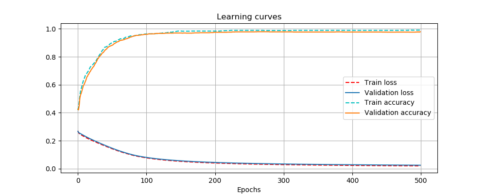 Learning curves of the network
Performance comparison with PyTorch
We run the training of the same model 20 times on a MacBook Pro (2.7 Ghz Intel Core i5) and compute the mean and median execution durations using Autogradlib and PyTorch.
| Library | Mean time | Median time |
|---|---|---|
| PyTorch | 0.804s | 0.779s |
| Autogradlib | 1.961s | 1.920s |
We observe that Autogradlib is only a bit more than twice as slow as PyTorch. However, we must notice that the heavy tensor operations are actually handled by PyTorch’s Tensor in both cases. Thus, the difference in execution time is mainly due to the fact that Autogradlib’s gradient operations graph is computed in Python, while PyTorch implements it in C from what I understood.
Conclusion
In this project, we show that by simply using the chain rule and a DAG structure, we can build a relatively powerful small deep learning framework.