Physically-based 3D renderer in C++

In this project, I wrote a complete 3D renderer in C++ and extended it with advanced features including image-based lighting and Subsurface scattering. Please find below my work in the context of the EPFL rendering competition from the course CS-440: Advanced Computer Graphics.

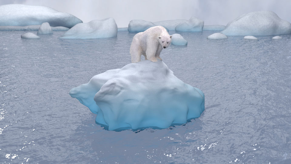
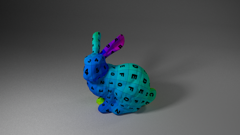
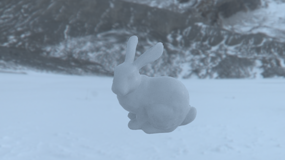
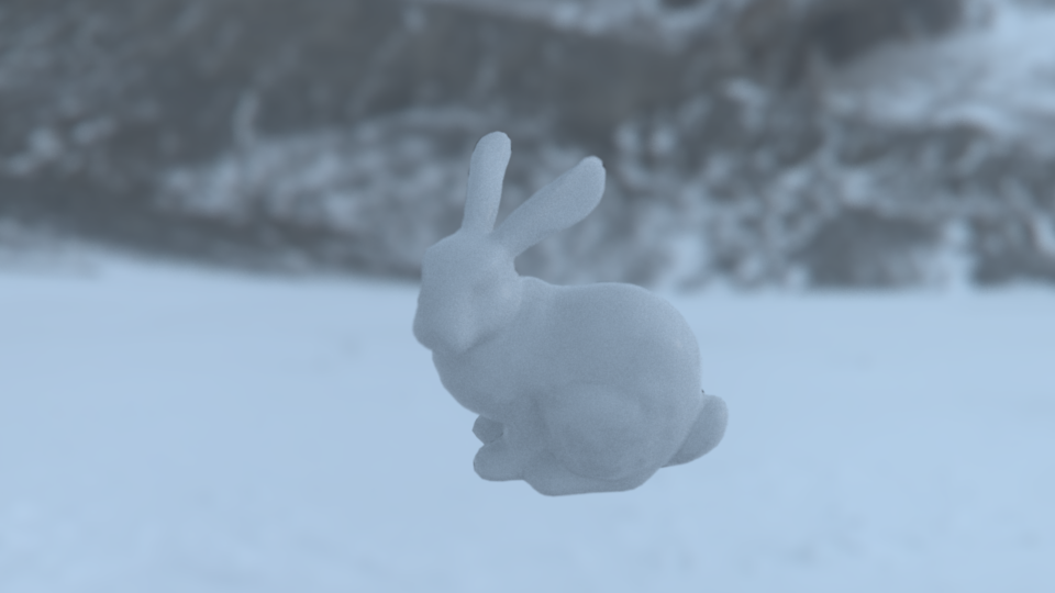
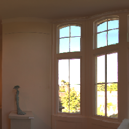
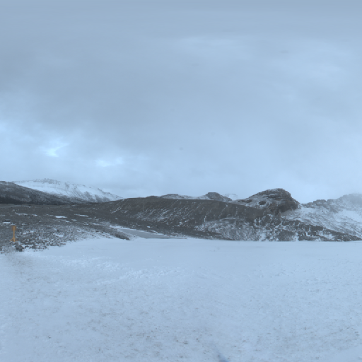
Motivational image

I understood the subject “The Last One” as an environmental message: global warming is an important and topical issue, causing a rapid decline in Artic sea ice over the last several decades. Polar bears are thus endangered and have been classified by the WWF as vulnerable (i.e. “faces a high risk of endangerment in the medium term”).

As a consequence, they might be the last ones in a near future if no measure against climate change is taken.

Implemented features

Note: all the test scenes shown below can be found in the `scenes/final` folder and can be reproduced.

Textures (10 points)

Code:

• include/nori/texture.h
• src/texture_const.cpp
• src/texture_img.cpp

We extend Nori with a new NoriObject called Texture. We write it as a template class so that it can be used both for colors and floats.

We then define the subclasses ConstTexture and ImageTexture (see texture_const.cpp and texture_img.cpp) so that a texture can be either defined with a bitmap image or with a constant color/float value.

Below, we compare the resulting rendering when applying an image texture in Blender and in Nori (all the Blender and XML files can be found in the scenes/final/texture/validation folder).

Applying it to a parquet texture, we get:

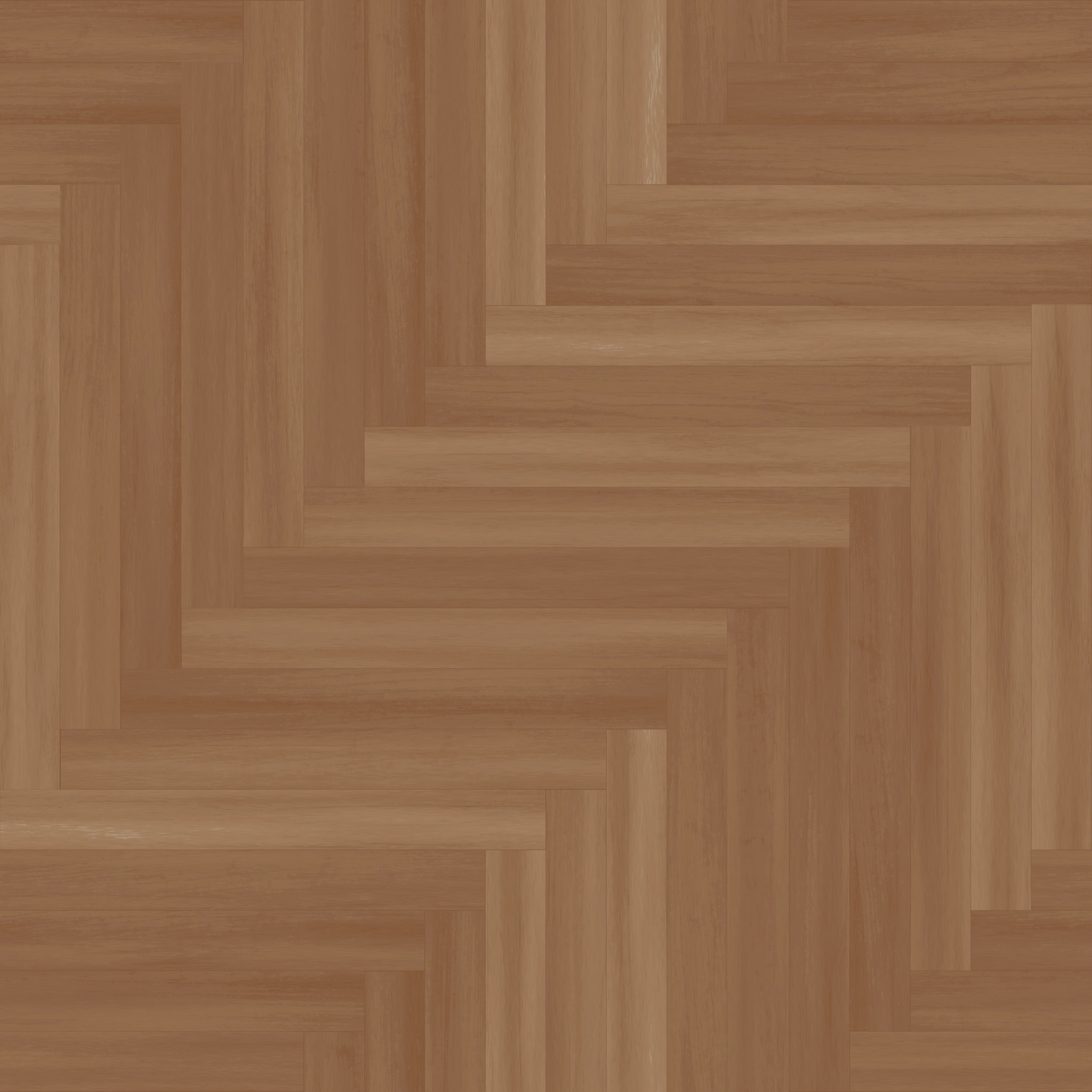
Parquet texture applied to the floor (scenes/final/texture/parquet)

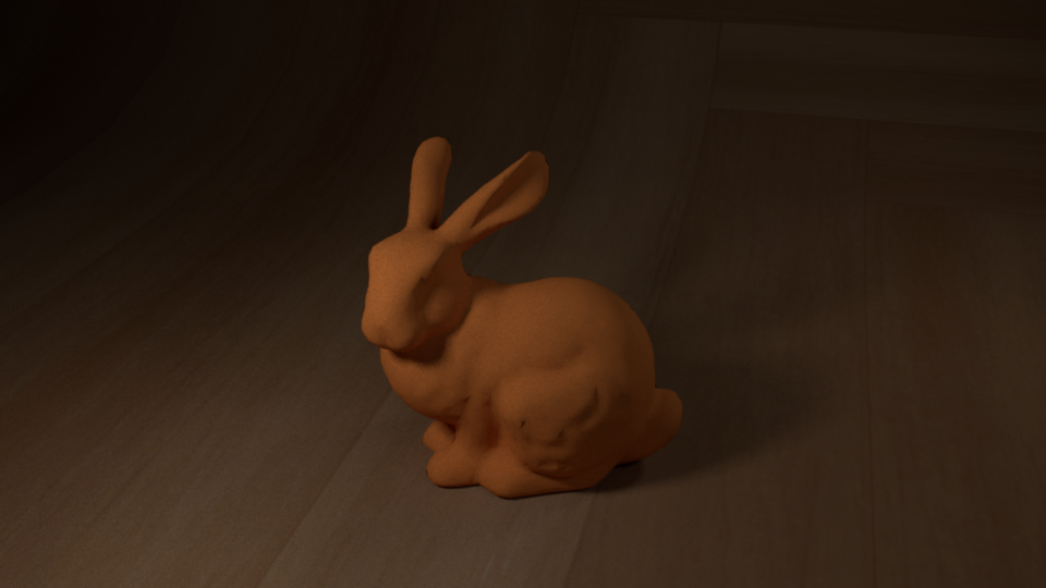
Bump mapping (10 points)

Code:

• include/nori/bsdf.h
• src/bsdf.cpp

We add the method BSDF::bump(Intersection *its, Texture<float> *bumpMap) which is responsible for modifying the normal frame at a given intersection point. Any subclass of BSDF is then free to call this function at ray-tracing time.

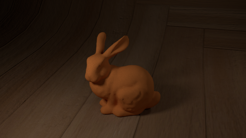
Bumpmap added to the parquet (scenes/final/bumpmap/parquet)

Depth of field (10 points)

Code:

• src/perspective.cpp

In just a few lines of code, we can extend Nori to simulate depth of field. I extended the Nori exporter Blender plugin by computing the distance between the in-focus object of Blender and the camera position to fill the focalDistance parameter.

Comparing different radius values for the depth of field feature (scenes/final/dof)

Mix BSDF (10 points)

Note: this feature wasn't part of list, I think 10 points is a good amount for the work it has required.

Code:

• ext/tinyexpr
• src/mix.cpp
• include/nori/formula_parser.h
• src/geometry_formula.cpp

In order to mix different materials like in Blender, we implement the new BSDF called Mix (see mix.cpp) that wraps two child BSDFs. The amount of each material to consider for the mixed one is determined by a factor (number between 0 and 1).

To make the factor vary with respect to some variables, we introduce a new NoriObject called FormulaParser responsible for parsing a given string representing a mathematical expression. Those variables can be anything related to the scene: e.g. coordinates of the intersection point, coordinates of the surface normal… I was mostly interested in the coordinates of the intersection point, so I implemented the geometry_formula.cpp file that is responsible for evaluating the provided formula at a given intersection point using the coordinates $x$, $y$ and $z$. Those numbers are wrapped into [0,1] using the Shape’s bounding box. In this way, the user can provide in the XML file any function from [0,1]^3 -> [0,1].

For the parser, we use the lightweight TinyExpr library.

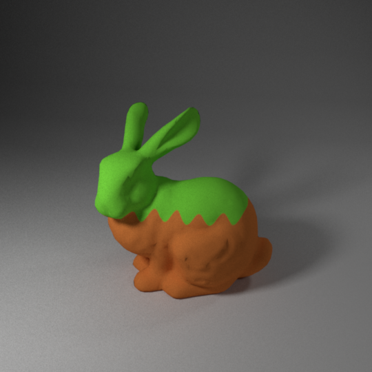
Some examples from scenes/final/geometry_mix:

Mix BSDF using the formula $z$

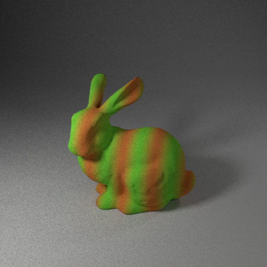Mix BSDF using the formula $\frac{1}{2} (\sin(2 \pi x 4) + 1)$

Mix BSDF using the formula $\frac{1}{1 + exp(-1000 (z - 0.5 + 0.03 \sin(2 \pi x 8) ))}$

Ray-intersection involving non-triangular shapes (20 points)

Code:

• include/nori/shape.h
• src/sphere.cpp
• src/curve.cpp

In order to render the polar bear’s fur efficiently, we implement the curve primitive. Until now, all the rendered objects were instances of the Mesh class, which stores a list of the triangles that define the mesh. We extend Nori by creating an abstract superclass called Shape (see shape.h) from which our new primitives will inherit.

We start by implementing the simple Sphere primitive (see sphere.cpp) defined by its center and radius.

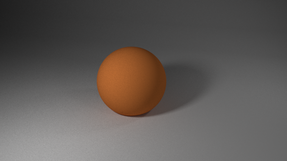A scene using the Sphere primitive (see scenes/final/sphere)

We then implement the Curve primitive. The underlying Bézier curve is defined by 4 control points $p_{0}$, $p_{1}$, $p_{2}$ and $p_{3}$ and is parametrized by $u \in [0, 1]$:

\[p(u) = (1-u)^{3}p_{0} + 3(1-u)^{2}up_{1} + 3(1-u)u^{2}p_2 + u^{3}p_{3}\]

Since our main goal is to apply it to the fur of a polar bear that is short, we can simplify a little the approach in the PBRT book (in particular we can store the full curve directly instead of splitting it in smaller pieces; however, for the ray intersection test, we still recursively test the intersection on sub segments since this increases the efficiency).

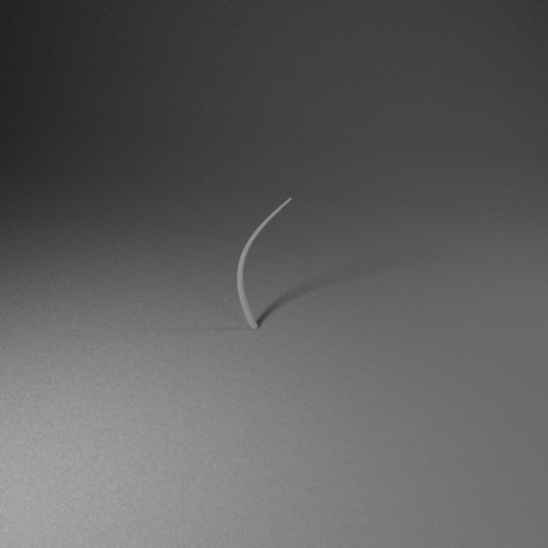A single Curve shape of type cylinder (see scenes/final/curve/curve)

Finally, in order to be able to render images with fur, I further extended the Nori exporter Blender plugin, by exporting automatically Cycle’s Hair particles.

Blender Cylces doesn’t use Bézier curves for Hair particles: instead, it uses linear segments (the default number, 6, can be increased). To export it to a Bézier curve, we make use of the fact that any series of any 4 distinct points $y_0$, $y_1$, $y_2$ and $y_3$ can be converted to a cubic Bézier curve that goes through all 4 points in order, using the following control points: \(p_0 = y_0\) \(p_1 = (-5y_0 + 18y_1 - 9y_2 + 2y_3 ) / 6\) \(p_2 = (2y_0 - 9y_1 + 18y_2 - 5y_3 ) / 6\) \(p_3 = y_3\)

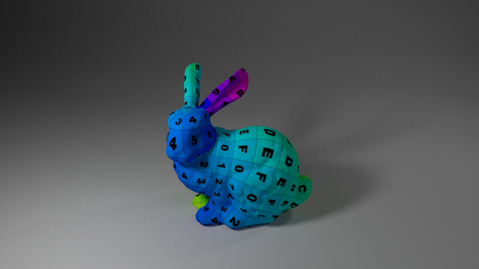
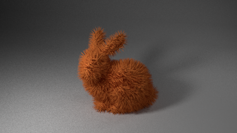Stanford Bunny rendered with 20,000 fur particles (see scenes/final/curve/fur)

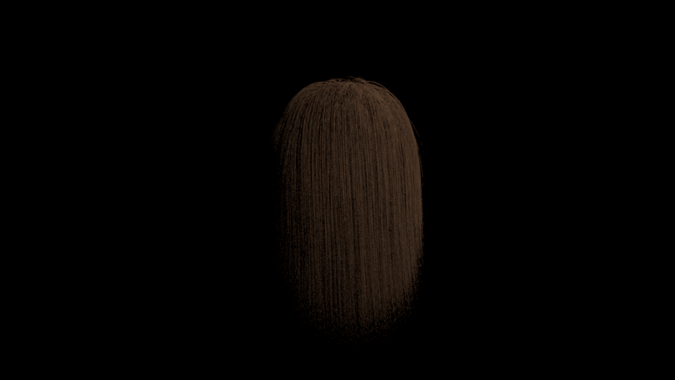Model with 5,000 diffuse hairs (see scenes/final/curve/hair)

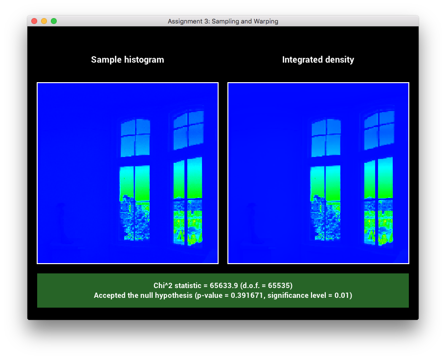
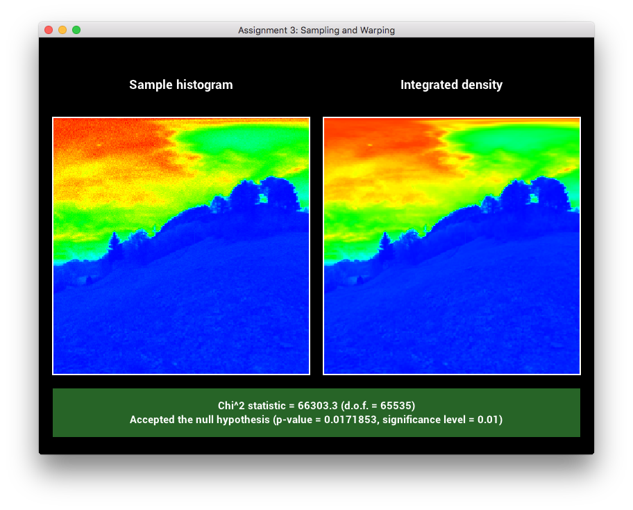
Image-based lighting (30 points)

Code:

• include/nori/image_light.h
• src/warp.cpp

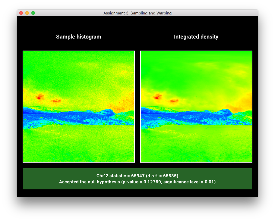
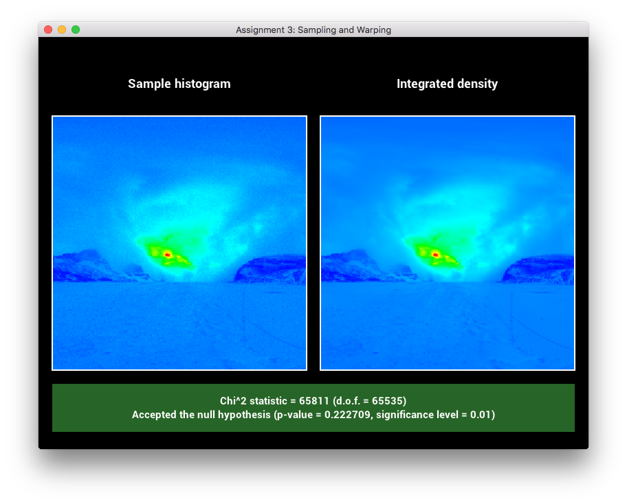
This feature has already been discussed in assignments 3 and 5. By using a power of 2 as the resolution of the Chi^2 test (here xRes, yRes = 256) and keeping the sampleCount at 1000 * res, we get the following Chi^2 results (see scenes/final/IBL/chi2):

In order to use Image Based Lighting with an image of any size, I slightly changed the implementation of the Bitmap class by finding the upper power of 2 of the original size of the image, and zero-padding it to the right and the bottom so that it fits this new dimension. E.g. an input image of size 240x510 will be zero-padded to fit the size 512x512.

Finally, we have to make sure that rays that leave the scene don’t intersect the black (zero-padded) region of the environment map, so we keep in memory the ratio between the original and new sizes of the image to warp the spherical coordinates accordingly (see the method ImageBasedLight::mapDirectionToPoint).

There was certainly a way to directly deal with aspect ratio in the Warp::squareToHSW function, but in this way the latter could remain unchanged.

A mirror sphere in an interior scene (see scenes/final/IBL/mirror)

Subsurface scattering (60 points)

Code:

• src/subsurface.cpp

Implementation

We implement the paper “A Rapid Hierarchical Rendering Technique for Translucent Materials”, Jensen, H.W. & Buhler, J. (2002), which combines the dipole approximation with a hierarchical data structure for an efficient evaluation of translucent materials. However, as advised by the teaching staff, I didn’t implement the Turk repulsion algorithm and enabled to increase the number of sample points by a certain factor with the samples_count_factor attribute, instead.

We first generate a certain number of points on the surface of the mesh. For an efficient computation at ray-tracing time, we store these points in an Octree structure (see the SubsurfaceOctree and OctreeNode structures in subsurface.cpp).

We then compute the irradiance by Monte Carlo estimation at each of the sampled locations, in parallel using TBB’s parallel_for function.

We can compute the irradiance at a given sample point by integrating the radiance over the hemisphere:

\[E(x) = \int_{H} L(x, \vec{\omega}) \cos \theta d \vec{\omega}\]

The subsurface scattering BSDF works differently from other BSDFs since the irradiance at a given intersection point has already been computed and we can terminate the Integrator’s ray. We extend BSDF with a function getSSSRadiance that is called by Integrator’s whenever the intersected material is translucent.

As many other rendering engines, we enable to specify a given scale. Indeed, the scattering and absorption coefficients are defined in a certain unit, which might not correspond to the unit of the scene; we simply multiply $\sigma_s$ and $\sigma_a$ by the provided scale. Below, we show the resulting teapot scene using subsurface scattering with two different scale values.

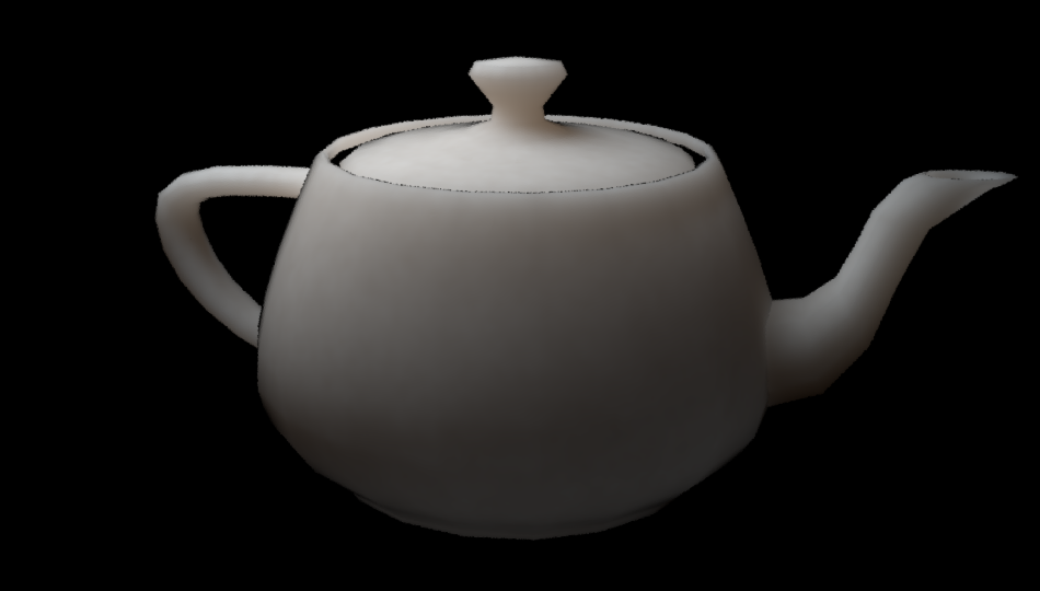
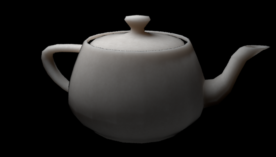
Comparing different scale values for the SSS feature (scenes/final/subsurface/teapot)

In order to add specular reflections to the scene, we can use our previously defined Mix BSDF to blend SSS and microfacet materials.

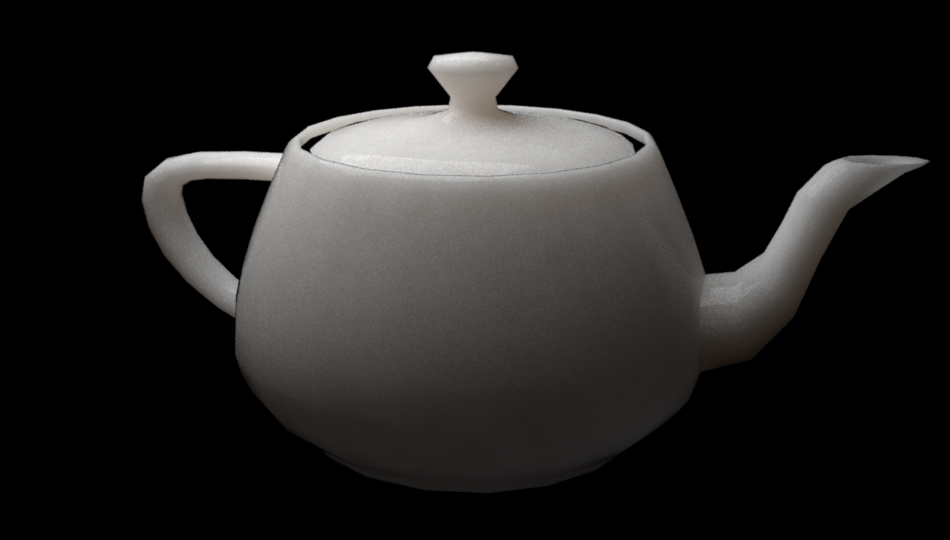Mix of SSS and microfacet materials (scenes/final/subsurface/teapot)

Finally, by setting $\sigma_a$ and $\sigma_s$ to some measured values from real objects (see “A Practical Model for Subsurface Light Transport”), we can render Marble, Ketchup or Apple-like materials:

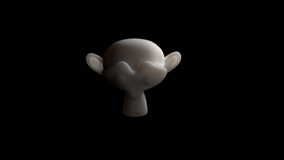
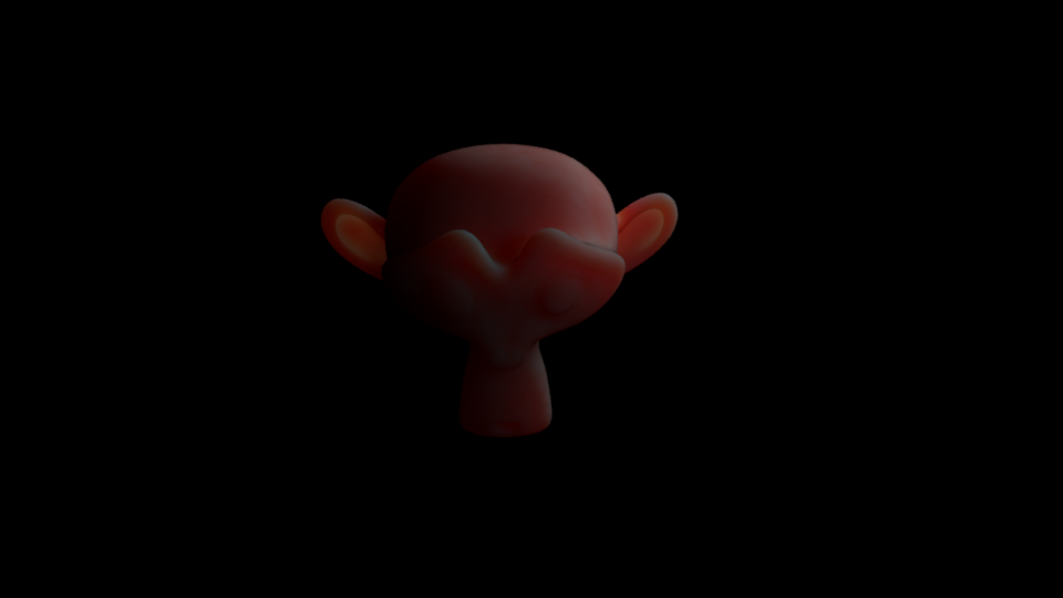
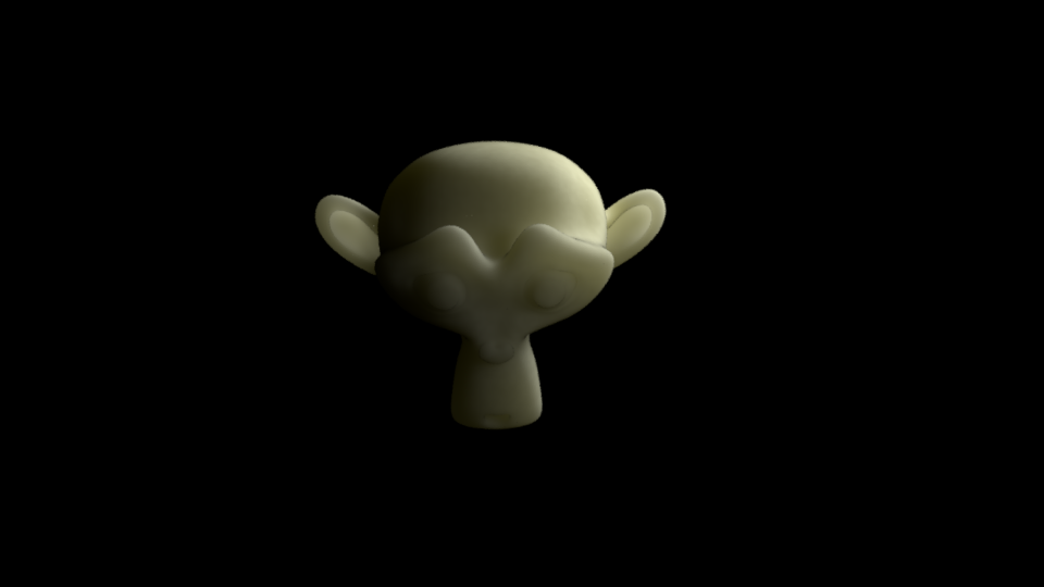
Comparing different $\sigma_a$ and $\sigma_s$ values for the SSS feature (scenes/final/subsurface/monkey)

Validation

The validation of this feature wasn’t easy: we cannot compare renderings with Blender’s ones since it uses different parameters than our physically based scattering and absorption coefficients and it most likely doesn’t implement the same paper. I ended up by building my own Student t-test with a carefully designed scene, where it is possible to compute the theoretical expected radiance received by a camera.

The scene is shown in the image below: the small sphere (radius = 0.1) in the center is a light emitter of (constant) radiance $L_e(x, \vec{\omega}) = L_e = 5$ and surface area $S_e = 4 \pi \cdot 0.1^2$. The large sphere (radius = 1) on the outside is the SSS material with $\sigma_s = 2$ and $\sigma_a = 0.002$. The camera is looking downwards.

The radiant exitance of the light emitter at a surface point is given by integrating its radiance over the hemisphere. When multiplying by the area, we finally get the total flux of this light emitter: $\pi L_e \times S_e$. Therefore, the average irradiance at each sample point is $\frac{\pi L_e \times S_e}{S}$, where $S$ is the surface of the mesh.

We want to compute the average radiance received by the camera in this setup. We know that $L_o = \frac{F_t(x, \vec{\omega})}{F_{dr}} \cdot \frac{M_o(x)}{\pi}$. But in this setup, the camera is centered in the sphere, so rays coming from the camera will be normal to the surface of the sphere: thus, $F_t(x, \vec{\omega})$ is constant. A simple computation from the Fresnel equations gives $F_r = (\frac{\eta_t - \eta_i}{\eta_t + \eta_i})^{2}$, with $\eta_t = 1.3$ and $\eta_i = 1.0$ here. Moreover, we have $F_{dr} = - \frac{1.440}{\eta^2} + \frac{0.710}{\eta} + 0.668 + 0.0636 \eta$. We then have at a point $x$:

\[M_o(x) = \int_{\text{sphere}} \frac{E(x_i) A(x_i)}{4 \pi} (1 - F_{dr}) \left(z_r (\sigma_{tr} + \frac{1}{d_r}) \frac{e^{-\sigma_{tr} d_r}}{d_r^{2}} + z_v (\sigma_{tr} + \frac{1}{d_v}) \frac{e^{-\sigma_{tr} d_v}}{d_v^{2}} \right) d x_i\]

where $r = \left\Vert x - x_i\right\Vert$, $z_r = l_u$, $z_v = l_u(1 + \frac{4}{3}A)$, $d_r = \sqrt{r^2+z_r^2}$ and $d_v = \sqrt{r^2+z_v^2}$.

But $E(x_i) = E = \frac{\pi L_e \times S_e}{S}$ is constant. We can therefore compute the simplified integral:

\(\int_{\text{sphere}} \left(z_r (\sigma_{tr} + \frac{1}{d_r}) \frac{e^{-\sigma_{tr} d_r}}{d_r^{2}} + z_v (\sigma_{tr} + \frac{1}{d_v}) \frac{e^{-\sigma_{tr} d_v}}{d_v^{2}} \right) d x_i\) \(= \frac{1}{2} \left( z_r \left( \frac{e^{-\sigma_{tr} z_r}}{z_r} - \frac{e^{-\sigma_{tr} \sqrt{z_r^{2} + 4}}}{\sqrt{z_r^{2} + 4}}\right) + z_v \left( \frac{e^{-\sigma_{tr} z_v}}{z_v} - \frac{e^{-\sigma_{tr} \sqrt{z_v^{2} + 4}}}{\sqrt{z_v^{2} + 4}}\right) \right)\)

Finally, we have:

\[L_o = \frac{(1 - F_r) \cdot (1 - F_{dr}) \cdot E \cdot S}{4 \pi \cdot F_{dr}} \times \frac{1}{2} \frac{z_r \left( \frac{e^{-\sigma_{tr} z_r}}{z_r} - \frac{e^{-\sigma_{tr} \sqrt{z_r^{2} + 4}}}{\sqrt{z_r^{2} + 4}}\right) + z_v \left( \frac{e^{-\sigma_{tr} z_v}}{z_v} - \frac{e^{-\sigma_{tr} \sqrt{z_v^{2} + 4}}}{\sqrt{z_v^{2} + 4}}\right)}{\pi}\] \[L_o \approx 0.03074166\]

We can now build a t-test XML file with this reference value (see scenes/final/subsurface/test). The test passes successfully with 10,000 samples!

Student t-test on the previously described scene

Summary

(80 points to get the best grade)

Feature	Points
Minor features
Textures	10 pts
Bump mapping	10 pts
Depth of field	10 pts
Mix BSDF	10 pts
Small features
Ray-intersection involving non-triangular shapes	20 pts
Medium features
Image based lighting	30 pts
Big features
Subsurface Scattering	60 pts
Total	150 pts

Final rendering

---