Deep Learning for Object Tracking

1. Introduction

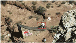
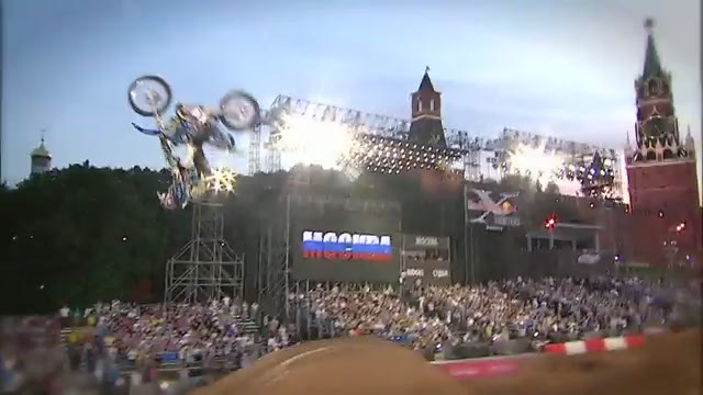
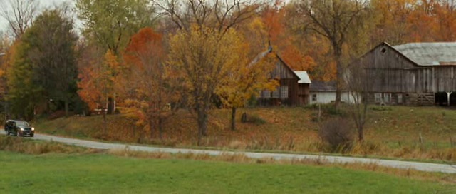
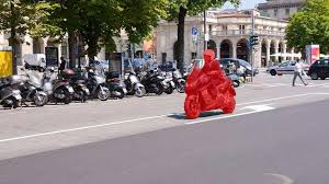
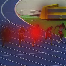
Visual object tracking is an important problem in computer vision consisting of tracking an object in any sequence, given only its first frame bounding box annotation. This is a hard task: indeed, to be successful, the tracker has to be class-agnostic, robust to severe appearance changes (rotations, lighting conditions, motion blur), to temporary occlusions and to semantic distractors. Benchmark datasets such as OTB-2015 (see figure 1) contain such challenging sequences.

Figure 1: A few frames from the OTB-2015 dataset: a challenging dataset including sequences with semantic distractors, occlusions, rotations, scalings and motion blur.

Several variants of the tracking problem can be found in the computer vision literature, including people tracking and semi-supervised video segmentation. The first variant consists of tracking one or multiple people in a scene. Since the tracker doesn’t need to be class-agnostic in this case, models usually employ the tracking by detection paradigm, which first passes the current frame to an object detector and then processes this output to perform the actual tracking. Such trackers are usually benchmarked on the MOTChallenge [Milan et al., 2016]. In the second variant, semi-supervised video segmentation, trackers are provided with a pixel-level segmentation of the initial frame and have to output the segmentation of the next frames. If the formulation resembles the one from the visual object tracking task, there are some differences including the facts that there is no ‘causal’ requirement (all the frames are provided at the beginning and can be analyzed before performing the tracking) and no real-time requirement (compared to object tracking whose VOT challenge has a separate competition for real-time trackers). Video segmentation trackers are usually benchmarked on the DAVIS Challenge [Perazzi et al., 2016], which contains only very short sequences (2-4 seconds, mean number of frames per sequence: 69.7) compared to benchmarks in object tracking (e.g. OTB, which has an average sequence length of about 20 seconds).

(a) People tracking

(b) Semi-supervised video segmentation

Figure 2: Illustration of two variants of the object tracking problem: people tracking and semi-supervised video segmentation.

In this project, we will analyze the current state-of-the-art real-time object trackers, aim to reproduce them and explore alternative network constructions to address some concerns that we might identify.

I have chosen to work on real-time tracking for my semester project since it is both a very exciting and difficult problem. What’s more, as the project formulation was very open and research-oriented compared to other more applied projects, it seemed to me as a good and challenging way to get started into research as a Master student in a competitive research branch.

Recent trackers can be divided in two categories: correlation filter-based trackers which make use of circular cross-correlation and perform operations in the Fourier domain, and deep trackers, which train a deep network to perform the tracking. Some works like [Danelljan et al., 2017] combine both approaches by using deep features in a correlation filter-based tracker. However, state-of-the-art trackers are computationally expensive and fail to track at real-time. Recently, exclusively offline-trained deep trackers have emerged, running in real-time and achieving competitive results. Since the aim of this project is real-time tracking, we will explore them in more details in the following.

2.1 Real-time trackers

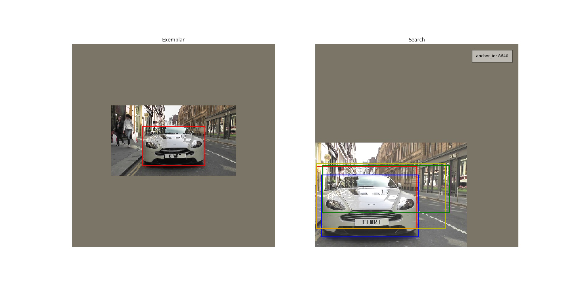
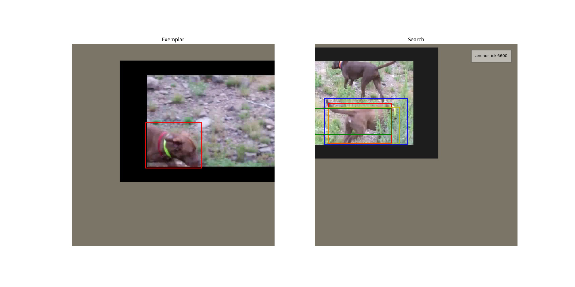
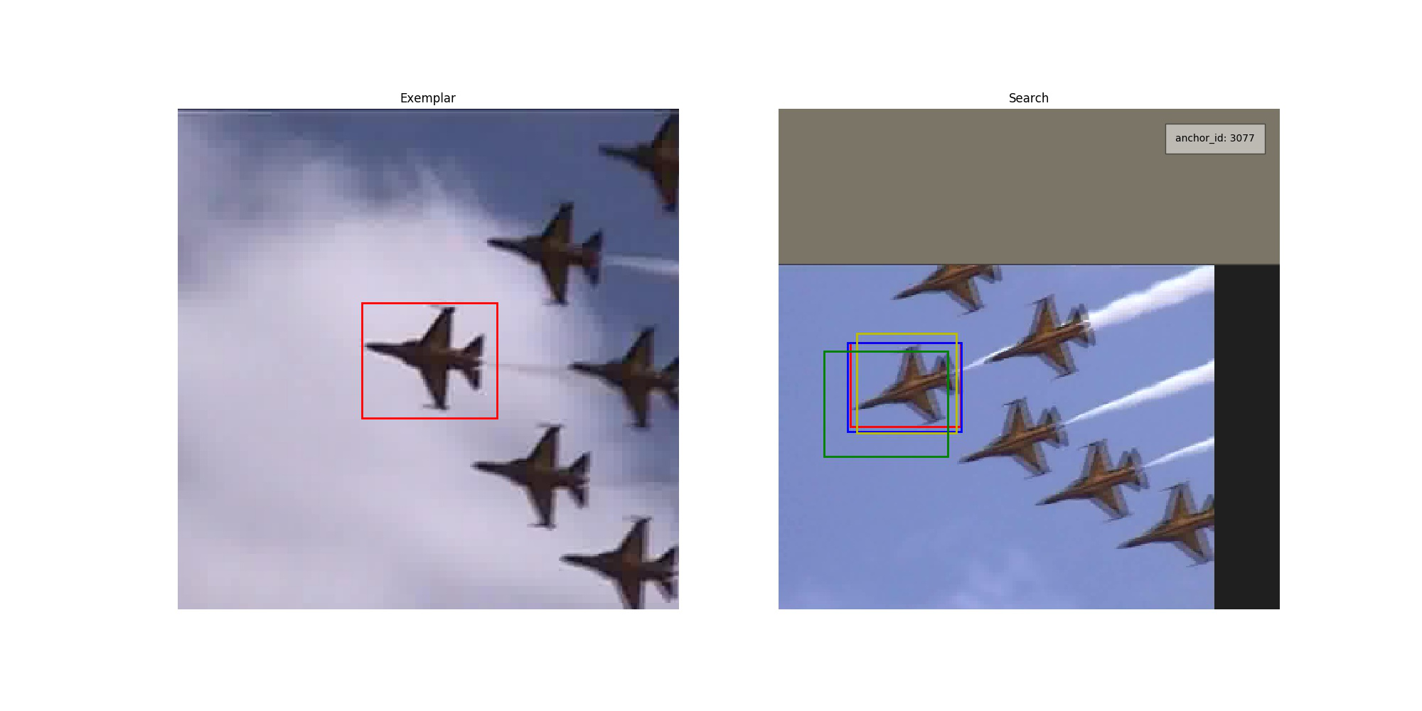
The work from [Bertinetto et al., 2016] has pioneered the real-time object tracking branch by introducing the idea of an offline-trained architecture that measures the similarity between two images. By making the architecture additionally fully convolutional, we can then compute the similarity score between an exemplar image and every subwindow of a large search image in a single forward pass, making the tracker run extremely fast. More precisely, as shown in figure 3, the Siamese network consists of two branches that process an exemplar frame $z$ of size $127 \times 127$ and a search image $x$ of size $255 \times 255$ using a shared conv-net $\varphi$. The branches result in two feature maps of same channel size that can be cross-correlated (operation $*$) to output a correlation map of size $17 \times 17$. This network can then be trained offline on a large dataset using cross-entropy loss.

Figure 3: The Siamese Fully Convolutional (SiamFC) tracker architecture [Bertinetto et al., 2016]. The network takes as input an exemplar frame $z$ and a search frame $x$ and outputs a correlation map representing the similariy score of the search image subwindows with the exemplar.

This idea has been further improved by the SiamRPN (Siamese Region Proposal Network) [Li et al., 2018b] tracker by separating the cross-correlation computation into two branches: one responsible for determining the best default bounding box (see the section 2.2 for more details), and another for regressing the offsets (position, width and height) of the selected default box. The architecture is shown in figure 4.

Figure 4: The SiamRPN architecture [Li et al., 2018b]. Similarly to [Bertinetto et al., 2016], the exemplar and search frames are first passed into a conv-net (here, a modified version of AlexNet). The resulting feature maps are then processed by two seperate branches: a classification branch which outputs a confidence score map for each one of the $k$ default boxes, and a regression branch, which outputs normalized offsets (noted $dx, dy, dw, dh$) at each location and for every default box.

More recently, the ATOM (Accurate Tracking by Overlap Maximization) [Danelljan et al., 2018] tracker has reached real-time state-of-the-art performance by combining both an online-trained classification network and an offline-trained estimation branch that estimates the overlap score between a given proposal and the ground-truth bounding box. The predicted bounding box can then be computed by gradient ascent in order to maximize this overlap score (see the architecture in figure 5).

Figure 5: The ATOM architecture [Danelljan et al., 2018]. The exemplar frame is processed by a ResNet network, followed by a convolutional layer and a Precise ROI Pooling layer using the ground-truth bounding box. Finally, a fully connected layer outputs two modulation vectors which are multiplied channel-wise in the branch processing the search frame. This branch is similar to the one used for the exemplar, except that the PrPool layers use a bounding box estimate instead of the ground-truth one.

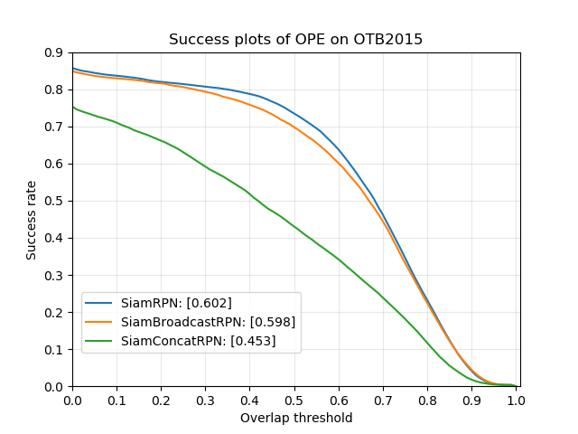
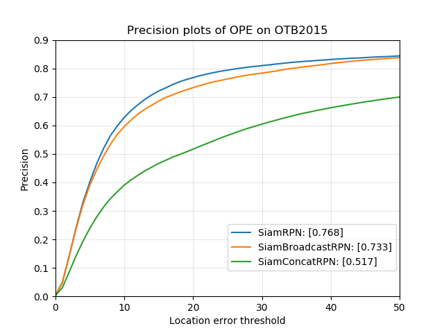
Finally, the SiamRPN tracker has been improved by two revisions: DaSiamRPN [Zhu et al., 2018] and very recently SiamRPN++ [Li et al., 2018a++], resulting in the new state of the art real-time tracker on both the OTB-2015 (see figure 7) and VOT-2018 datasets (see table 1).

Figure 6: The SiamRPN++ architecture [Li et al., 2018a]. Multiple SiamRPN blocks are computed from features learned at different levels of a ResNet network and aggregated into a regression and classification map. Cross-correlation layers are moreover replaced by depth-wise correlation structures, similarly to [Wang et al., 2018].

Figure 7: Comparison of the success and precision plots with the state-of-the-art trackers on the OTB-2015 dataset.

	DLSTpp	DaSiamRPN	SASiamR	CPT	DeepSTRCF	DRT	RCO	UPDT	SiamRPN	MFT	LADCF	ATOM	SiamRPN++
EAO	0.325	0.326	0.337	0.339	0.345	0.356	0.376	0.378	0.383	0.385	0.389	0.401	0.414
Acc.	0.543	0.569	0.566	0.506	0.523	0.519	0.507	0.536	0.586	0.505	0.503	0.590	0.600
Robust.	0.224	0.337	0.258	0.239	0.215	0.201	0.155	0.184	0.276	0.140	0.159	0.204	0.234

Table 1: Comparison with the state-of-the-art in terms of expected average overlap (EAO), accuracy and robustness (failure rate) on the VOT2018 benchmark. Best score shown in bold.

2.2 Object Detection

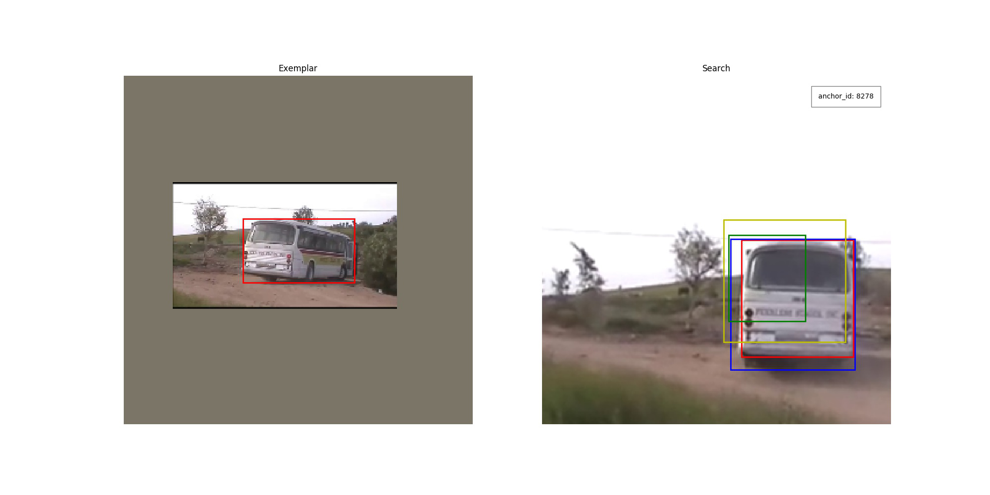
Even if we will not use the tracking by detection paradigm, it might be useful to borrow some ideas from the object detection literature and apply them to object tracking. In particular, we will extensively use the concept of default or anchor boxes introduced by [Redmon et al., 2016] and [Liu et al., 2016] in order to detect objects of different aspect ratios and scales. As shown in figure 8, bounding box proposals are generated from several feature maps of decreasing spatial dimension, corresponding to an increasing receptive field, thus enabling to detect objects of increasingly large scale. In figure 9, we illustrate the fact that in a feature map of dimension $m \times n$, each grid cell encodes the center of one or more default boxes: e.g. in the SSD architecture, we define 6 default boxes (2 boxes of aspect ratio 1:1 and one box each for the aspect ratios 2:1, 3.1, 1:2 and 1:3).

Figure 8: The SSD architecture [Liu et al., 2016]. Bounding box proposals are generated from several feature maps of decreasing spatial dimension.

Figure 9: Default boxes as used in SSD. For every feature map (here $8 \times 8$) and at every feature map location center, we define 6 default boxes: 5 boxes of scale $s_k$ at each aspect ratio 1:1 (in blue), 2:1, 1:2 (in orange), 3.1 and 1:3 (in grey) and one square box of scale $s_k'$ (in green).

More specifically, at the $k^{\text{th}}$ feature map, we define the scale values $s_k$ and $s_k’$. For every aspect ratio value $a \in {1, 2, 3, \frac{1}{2}, \frac{1}{3}}$, the associated default box has width and height:

\[\left\{ \begin{array}{l} w = s_k \sqrt{a} \\ h = \frac{s_k}{a} \end{array} \right.\]

so that its area is $w \times h = s_k^2$. Finally, we add the 1:1 default box of scale $s_k’$ (the green one on figure 9).

3. My work

3.1 Reproducing SiamRPN: implementation details

During the first part of my semester work, my aim was to reproduce the results obtained in [Li et al., 2018b]. Since the repository github.com/foolwood/DaSiamRPN only includes the tracking code, it cannot be used as a base to build alternative networks.}. We write below some implementation details. The code is written using PyTorch 0.4.

Datasets: We use several datasets for the training (PyTorch makes it easy to concatenate different datasets and train a network by sampling simultaneously from them): similarly to [Li et al., 2018b], we use the ILSVRC2015 VID dataset [Russakovsky et al., 2015] containing 3,862 train videos for a total of 1.3 million frames. Instead of using additionally the Youtube-BoundingBoxes dataset, we train our network on TrackingNet [Müller et al., 2018] which is based on YT-BB: it contains a total of 30,132 sequences, representing 14,431,266 frames; however, only 6 chunks out of 12 were downloaded in order not to saturate the storage capacity of the CVLAB server. Both of these datasets have a limited number of categories (around 30), which can result in a bias of the tracker which will not be trained to recognize unseen classes of objects. We thus implement a synthetic data procedure based on the COCO dataset [Lin et al., 2014] which contains 91 categories and 328,000 images: to also improve the robustness of the tracker against semantic distractors, we add semantic distractors to each search frame, i.e. an object of the same semantic class as the target. Since the COCO dataset includes segmentation annotations, it is easy to crop only this object from another image; we finally randomly position this distractor in the search image, by constraining the IoU with the ground-truth bounding box, so that it doesn’t completely occlude the target. See figure 10 for a visualization of this procedure.

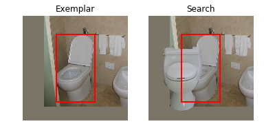
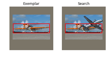
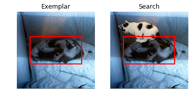
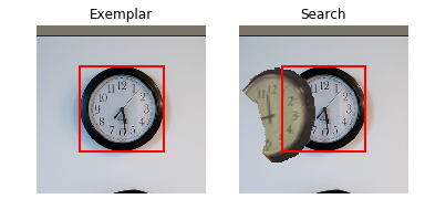
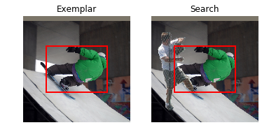
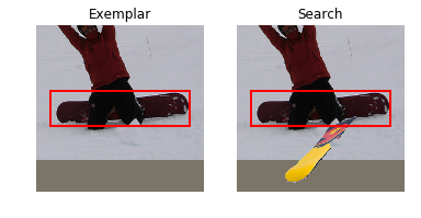
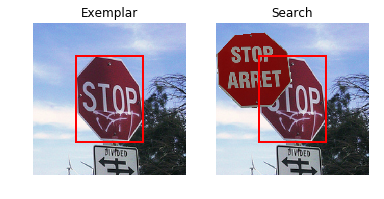
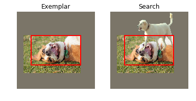
Figure 10: Some synthetic pairs including semantic distractors generated from the COCO dataset.

Image cropping: In order to deal with different aspect ratios of the object and have an input of constant size, we adopt the following image cropping strategy: as illustrated in figure 11, given a bounding box $(w, h)$, we compute the context $c = \texttt{context_amount} \cdot (w + h) / 2$, where $\texttt{context_amount}$ is equal to $0.5$ for the exemplar and $1.5$ for the search image. We then define $W = w + 2 c$ and $H = h + 2 c$; the area to crop is then the square of size $s = \sqrt{W \times H}$. Finally we resize the obtained region to 127 pixels for the exemplar and 255 pixels for the search image.

Figure 11: Illustration of the image cropping procedure used by the tracker. The image is cropped along the blue window of size $s$, which is resized to 127 pixels for the exemplar and 255 pixels for the search image.

The loss: The loss is defined in a similar way to [Liu et al., 2016], but instead of having different object classes, we only want to classify positive matches (the ground-truth object location) from negative matches (the background). To do so, we define $D$ default (or anchor) boxes $d_i$ ($i \in {0, \dots, D-1}$): $d_i = (d_i^{cx}, d_i^{cy}, d_i^{w}, d_i^{h})$ and one ground-truth bounding-box: $g = (g^{cx}, g^{cy}, g^{w}, g^{h})$. Then, for every default box index $i$, we further define:

the normalized ground-truth bounding-box $\hat{g_i}$:

\[\left\{ \begin{array}{l} \hat{g_i}^{cx} = (g^{cx} - d_i^{cx}) / d_i^w, ~~ \hat{g_i}^{cy} = (g^{cy} - d_i^{cy}) / d_i^h \\ \hat{g_i}^{w} = \log(\frac{g^w}{d_i^w}), ~~ \hat{g_i}^{h} = \log(\frac{g^h}{d_i^h}) \end{array} \right.\]

the matching indicator (default boxes which have an IoU in $\left]\delta_{\text{low}}, \delta_{\text{high}}\right[$ are not taken into account in the loss): $x_i = \left\{ \begin{array}{cll} 1 & \text{if } \text{IoU}(d_i, g) \geq \delta_{\text{high}} & \text{(positive match)}\\ 0 & \text{if } \text{IoU}(d_i, g) \leq \delta_{\text{low}} & \text{(negative match)} \end{array} \right.$
and the network output: confidence score $c_i \in \left[0, 1\right]$ and offset location prediction $l_i = (l^{cx}, l^{cy}, l^{w}, l^{h})$.

The loss is then simply defined by combining a classification and a regression term:

\[L(x, c, l, g) = \frac{1}{N} (L_{\text{conf}}(x, c) + \alpha L_{\text{loc}}(x, l, g))\]

where $\alpha$ is a hyper-parameter (fixed to 1.5 in the code) and

\[\left\{ \begin{array}{l} L_{\text{conf}}(x, c) = \text{BinaryCrossEntropyLoss}(c, x)\\ L_{\text{loc}}(x, l, g) = \sum_{i: x_i = 1} \text{smooth}_{L1}(l_i - \hat{g_i}) \end{array} \right.\]

Hard negative mining: Because of the heavy class imbalance (by the choice of $\delta_{\text{high}} = 0.55$, there are much more negative matches than positives), we impose a fixed ratio num_negatives / num_positives = 3. We moreover adopt the hard negative mining approach [Shrivastava et al., 2016] that consists of choosing the negative matches as the ones that contribute the most to the confidence loss.

Training: We train the network during 100 epochs (in one epoch, we sample one exemplar/search pair per sequence) with a batch size of 16 and a learning rate of $10^{-3}$ which is multiplied by a factor of 0.99 every 1000 training steps. The training is monitored using Tensorboard: we display different metrics of the train dataset (confidence loss, regression loss, total train loss, positive accuracy and negative accuracy) and compute the validation IoU on a validation set of approximately 500 sequences every epoch.

Tracking engineering: Similarly to SiamRPN [Lietal.,2018b], during tracking , we employ a strategy that suppresses large displacements by multiplying the correlation map score by a cosine window, as illustrated in figure 12. Additionally, we penalize scale changes using the penalty $e^{k \max(\frac{r’}{r}, \frac{r}{r’}) \max(\frac{s’}{s}, \frac{s}{s’})}$ where $r$ and $s$ represent the ratio and scale of the current prediction, and the values of the last frame are noted with a prime symbol.

(a) Exemplar

(b) Search

(d) Cosine window

(e) Correlation map

Figure 12: Visualization of applying a cosine window to the correlation map. The confidence scores are re-ranked after this procedure in order to suppress large displacements.

3.2 Other approaches

Even if the original SiamRPN tracker achieves very competitve results, as shown in [Li et al., 2018b] and that using a correlation map seems to be a good way to compute confidence scores, it is conceptually not clear why one could regress bounding boxes from it: intuitively, we need more information than a 2D map to infer precisely the shape of an object. What’s more, the ground-truth bounding box from the exemplar frame is used only to crop the image with the correct context amount and the ground-truth aspect ratio in particular is never used: we can therefore expect better results if our model includes this information. As a response to those remarks, we design two new architectures that should improve the results we got with the SiamRPN model.

SiamConcatRPN:: Inspired by the reference-guided mask propagation approach used in [Oh et al., 2018] for video segmentation, we build the network shown in figure 13. Notice that unlike all previous siamese architectures, the exemplar and search input frames have the same size. The purpose is two extract, using a ResNet50 backbone, identically shaped feature maps that we can then concatenate channel-wise and perform convolution operations on top of it. We use global convolution, as introduced in [Peng et al., 2017], by combining a $1 \times 9$ followed by a $9 \times 1$ convolutional layer with a $9 \times 1$ followed by a $1 \times 9$ convolution. The goal of this block is to match corresponding features between the exemplar and the search features: by using global convolution, we have an increased receptive field view compared to a simple $3 \times 3$ convolutional layer by only doubling the needed number of parameters. One Refine module is added by upsampling the feature map and fusing it with ResNet features from the search image, in order to double the feature map size and overcome the coarse representation of the scene. Finally, extra feature layers are used as in SSD to output both confidence and localization scores.

This architecture addresses the issue of SiamRPN in the sense that the proposals are generated from a feature map of channel size 512. However, it still doesn’t make use of the ground-truth bounding box of the exemplar frame. To do so, we represent the bounding box as a binary mask, use an additional convolutional layer and add the resulting feature map to the first layer of the ResNet50 network, as shown in figure 15a.

The same procedure is used for the search image. However, in this case, we don’t have the ground-truth bounding box at tracking time; we therefore use the predicted bounding box from the previous frame to guide the network. During training, naively using the ground-truth bounding box from the previous frame would result in a good train loss but a bad test loss since the predicted proposal may not be exactly at the true position: in order to make the network robust to these errors, we add some jitter (both in position and size) to the ground-truth bounding box, as shown in figure 15b. Results are shown in section 4.

Figure 13: The SiamConcatRPN architecture. The exemplar and search feature maps are concatenated and processed by a global convolution block. The resulting feature map is refined and passed to the final RPN layers.

Figure 14: k × k Global convolution compared to a standard k × k convolutional layer.

(a) Exemplar frame

(b) Search frame

Figure 15: Illustration of how the ground-truth exemplar and search bounding boxes are used in the SiamConcatRPN architecture to produce a binary mask. The latter is processed by a convolutional layer and added to the first layer of the ResNet network.

SiamBroadcastRPN:: One of the issues of the architecture described above is that it is relying only on convolutional layers and may be missing a similarity map output. A way to address this problem is to reduce the exemplar feature map of size $H \times W \times C$ to a single vector of dimension $C$ using a MaxPool operation; then, instead of convolving this vector with the search feature map directly (which would result in a 2D correlation map), we broadcast the vector to the same spatial size as the search feature map, similarly to [Lu et al., 2018]. We can then concatenate the two feature maps as in the SiamConcatRPN architecture and output the confidence and localization scores using extra feature layers in an SSD-like fashion, as illustrated in figure 16. By doing this, the convolutional layers compute a similarity measure at every location of the search feature map, using a compact representation of the exemplar frame. Results are shown in section 4.

Figure 16: The SiamBroadcastRPN architecture. A MaxPool layer reduces the exemplar features to a vector, which can be concatenated to the search features after a Broadcast operation.

4. Results on OTB-2015

The networks described in section 3 are benchmarked on the OTB-2015 dataset in figure 17.

SiamRPN:: The reproduction of SiamRPN achieves a slightly lower success score than the original model [Li et al., 2018b] (which scores at 0.63 on OTB-2015). One possible reason is that the network was trained on the TrackingNet dataset (and moreover only half of it), which is a filtered version of the Youtube-Bounding Boxes dataset [Müller et al., 2018], while the original model was trained using Youtube-BB.

SiamConcatRPN:: While validation results are surprisingly good (see figure 18), the results on OTB-2015 are below expectations. We identify two possible explanations: the first one is that since the network is trained with jittered guides, it has a tendency to regress the bounding box of the closest semantic object: as an example, by choosing as exemplar a subpart of an object (like the lower half of a face or the window of a car), the network will end up tracking the entire object, resulting in a much lower IoU. Secondly, the network may place too much importance on the mask guide: thus, detecting the wrong semantic object in one frame will prevent the network from finding the true object in the next frames, resulting in a low robustness.

SiamBroadcastRPN:: The success score is very similar to the one obtained for SiamRPN. This is actually rather surprising since the architectures are completely different: indeed, instead of computing the cross-correlation (product) between two image patches, using their concatenated features only can achieve as good results.

Figure 17: Success and Precision plots of the constructed networks on OTB-2015.

Figure 18: Validation results from the SiamConcatRPN model after training. Each image pair corresponds to an exemplar and search frame. In the search image, the bounding boxes correspond to: the ground-truth (in blue), the predicted box (in red), the best default box (in yellow), the jittered guide (in green). On the top images, we identify that the network achieves to recover the bounding box of an object even when the guiding mask is severely scaled and displaced. On the bottom images, we notice that the guide is useful to distinguish the object from semantic distractors.

5. Conclusion

In this project, our aim was to reproduce state-of-the-art real-time trackers and explore alternative constructions. We successfully achieved almost state-of-the-art performance and built another network architecture resulting in a similar score. This project was also an extremely enriching experience for me, as it was one of my first real-world applications of the theoretical knowledge I had acquired in classes like Machine Learning, Deep Learning and Computer Vision during my first year at EPFL. Throughout this project, I have learned to implement and use object detectors like SSD, write maintainable code for the training of deep networks, monitor trainings using tools like Tensorboard, write complex data augmentation procedures, design and implement new networks, and acquired more transversal skills like reading very recent deep learning papers.

On a side note, recent trackers rely, as we have seen, on more and more complex training and data augmentation procedures; thus reproducing the published results has become both time-consuming and error-prone. Sharing complete codes of state-of-the-art networks (instead of only submitting tracking codes) would certainly be very beneficial for the tracking research community.

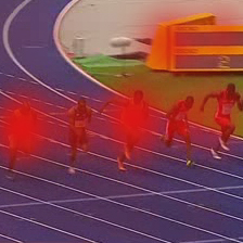
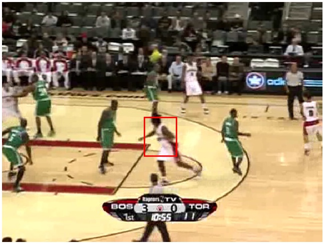
Finally, it is worthwhile noting that even if state of the art trackers have recently shown impressive performance, most of them if not all still fail on sequences that would seem easy for humans. This is particularly the case for sequences including temporary occlusions and semantic distractors (see figure 19), where humans have no difficulty to predict the trajectory of an object, in order to estimate its position when it is occluded, or to distinguish it from distractors. Thus, there is still room for improvement in the object tracking discipline, in contrast for instance to the object classification problem where human’s ability to classify has been outperfomed by deep networks: indeed, an approximate upper-bound on human error on the ILSVRC testset is 5.1% (karpathy.github.io/), compared to the state of the art 2.25% with the Squeeze-and-Excitation Resnet architecture [Hu et al., 2017]. One possible way of improvement would be to explicitly model the motion of the tracked object and include it in the tracker, or to follow an approach similar to [Luc et al., 2018] in order to predict future instance segmentations.

(a) Bird1

(b) Basketball

Figure 19: Failures of SiamRPN++ on the OTB-2015 dataset. Although the performance of this tracker is impressive, there is still room for improvement. In particular, SiamRPN++ fails in some sequences including occlusions and semantic distractors.

6. Acknowledgment

I would like to thank my supervisors, Dr. Erhan Gundogdu and Joachim Hugonot, for their availability, their kindness and their precious help throughout this semester work. I also thank them for giving me the opportunity to work on such an exciting and enriching project that gave me a glimpse of what research in deep learning is like. Finally, I want to thank the Computer Vision laboratory of the EPFL for giving me access to the lab’s infrastructure and computing power, enabling graduate students to work in the best possible conditions.

References

[Bertinetto et al., 2016] Bertinetto, L., Valmadre, J., Henriques, J. F., Vedaldi, A., and Torr, P. H. (2016). Fully-convolutional siamese networks for object tracking. In European conference on computer vision, pages 850–865. Springer.

[Danelljan et al., 2018] Danelljan, M., Bhat, G., Khan, F. S., and Felsberg, M. (2018). Atom: Accurate tracking by overlap maximization. arXiv preprint arXiv:1811.07628.

[Danelljan et al., 2017] Danelljan, M., Bhat, G., Khan, F. S., Felsberg, M., et al. (2017). Eco: Efficient convolution operators for tracking. In CVPR, volume 1, page 3.

[Hu et al., 2017] Hu, J., Shen, L., and Sun, G. (2017). Squeeze-and-excitation networks. arXiv preprint arXiv:1709.01507, 7.

[Li et al., 2018a] Li, B., Wu, W., Wang, Q., Zhang, F., Xing, J., and Yan, J. (2018a). SiamRPN++: Evolution of Siamese Visual Tracking with Very Deep Networks. arXiv preprint arXiv:1812.11703.

[Li et al., 2018b] Li, B., Yan, J., Wu, W., Zhu, Z., and Hu, X. (2018b). High Performance Visual Tracking With Siamese Region Proposal Network. In Proceedings of the IEEE Conference on Computer Vision and Pattern Recognition, pages 8971–8980.

[Lin et al., 2014] Lin, T.-Y., Maire, M., Belongie, S., Hays, J., Perona, P., Ramanan, D., Dollár, P., and Zitnick, C. L. (2014). Microsoft coco: Common objects in context. In European conference on computer vision, pages 740–755. Springer.

[Liu et al., 2016] Liu, W., Anguelov, D., Erhan, D., Szegedy, C., Reed, S., Fu, C.-Y., and Berg, A. C. (2016). Ssd: Single shot multibox detector. In European conference on computer vision, pages 21–37. Springer.

[Lu et al., 2018] Lu, E., Xie, W., and Zisserman, A. (2018). Class-agnostic counting. arXiv preprint arXiv:1811.00472.

[Luc et al., 2018] Luc, P., Couprie, C., Lecun, Y., and Verbeek, J. (2018). Predicting future instance segmentations by forecasting convolutional features. arXiv preprint arXiv:1803.11496.

[Milan et al., 2016] Milan, A., Leal-Taixé, L., Reid, I., Roth, S., and Schindler, K. (2016). Mot16: A benchmark for multi-object tracking. arXiv preprint arXiv:1603.00831.

[Müller et al., 2018] Müller, M., Bibi, A., Giancola, S., Al-Subaihi, S., and Ghanem, B. (2018). Trackingnet: A large-scale dataset and benchmark for object tracking in the wild. arXiv preprint arXiv:1803.10794.

[Oh et al., 2018] Oh, S. W., Lee, J.-Y., Sunkavalli, K., and Kim, S. J. (2018). Fast video ob- ject segmentation by reference-guided mask propagation. In 2018 IEEE/CVF Conference on Computer Vision and Pattern Recognition, pages 7376–7385. IEEE.

[Peng et al., 2017] Peng, C., Zhang, X., Yu, G., Luo, G., and Sun, J. (2017). Large kernel mat- ters—improve semantic segmentation by global convolutional network. In Computer Vision and Pattern Recognition (CVPR), 2017 IEEE Conference on, pages 1743–1751. IEEE.

[Perazzi et al., 2016] Perazzi, F., Pont-Tuset, J., McWilliams, B., Van Gool, L., Gross, M., and Sorkine-Hornung, A. (2016). A benchmark dataset and evaluation methodology for video ob- ject segmentation. In Proceedings of the IEEE Conference on Computer Vision and Pattern Recognition, pages 724–732.

[Redmon et al., 2016] Redmon, J., Divvala, S., Girshick, R., and Farhadi, A. (2016). You only look once: Unified, real-time object detection. In Proceedings of the IEEE conference on computer vision and pattern recognition, pages 779–788.

[Russakovsky et al., 2015] Russakovsky, O., Deng, J., Su, H., Krause, J., Satheesh, S., Ma, S., Huang, Z., Karpathy, A., Khosla, A., Bernstein, M., et al. (2015). Imagenet large scale visual recognition challenge. International Journal of Computer Vision, 115(3):211–252.

[Shrivastava et al., 2016] Shrivastava, A., Gupta, A., and Girshick, R. (2016). Training region- based object detectors with online hard example mining. In Proceedings of the IEEE Conference on Computer Vision and Pattern Recognition, pages 761–769.

[Wang et al., 2018] Wang, Q., Zhang, L., Bertinetto, L., Hu, W., and Torr, P. H. (2018). Fast online object tracking and segmentation: A unifying approach. arXiv preprint arXiv:1812.05050.

[Zhu et al., 2018] Zhu, Z., Wang, Q., Li, B., Wu, W., Yan, J., and Hu, W. (2018). Distractor-aware siamese networks for visual object tracking. In European Conference on Computer Vision, pages 103–119. Springer.