Quantum Amplitude Amplification and Estimation
Report: quantum_ampl_estimation.pdf
I’ve read the (very dense!) paper Quantum Amplitude Amplification and Estimation by Brassard et al. (2000) and made a comprehensible 30 minutes presentation.
I. Introduction
-
Given a set $X = {0, 1, \dots N-1}$ and a boolean function $\chi: X \longrightarrow {0, 1}$, we want to find a good element, i.e. an $x \in X$ such that $\chi(x) = 1$.
-
If there is only one good element, a classical search algorithm has an average complexity of $\sum_{i=1}^{N} i \times \frac{1}{N} = \frac{N+1}{2}$.
-
Quantum approach: given an equal superposition of states $\ket{\Psi} = \frac{1}{\sqrt{N}} \sum_{x = 0}^{N-1} \ket{x}$, if we measure $\ket{\Psi}$, we get the correct $\ket{x}$ with probability $1/N$: so, the average number of iterations is $N$.
-
Grover’s algorithm: we can transform $\ket{\Psi}$ in $\mathcal{O}(\sqrt{N})$ iterations so that performing a measurement on it gives the correct $\ket{x}$ with high probability.
-
Amplitude amplification is a generalization of Grover’s algorithm where the input is given as an arbitrary superposition of elements of $X$: $\ket{\Psi} = \mathcal{A} \ket{0} = \sum_{x \in X} \alpha_x \ket{x}$ and more than one element may be good elements.
-
We can write: \(\ket{\Psi} = \sum_{x: \chi(x) = 1} \alpha_x \ket{x} + \sum_{x: \chi(x) = 0} \alpha_x \ket{x} = \ket{\Psi_1} + \ket{\Psi_0}\) with $a = \braket{\Psi_1}{\Psi_1} \ll 1$ is the probability that measuring $\ket{\Psi}$ produces a good state.
-
The standard approach would thus need to iterate $1/a$ times to find a good state. Amplitude amplification enables a quadratic speed-up in $\mathcal{O}(1/\sqrt{a})$.
II. Quantum amplitude amplification
The amplitude amplification operator
-
$\ket{\Psi} = \mathcal{A} \ket{0} = \ket{\Psi_1} + \ket{\Psi_0}$.
-
$S_\chi$ is the oracle function: \(\ket{x} \longmapsto \left\{ \begin{array}{rl} -\ket{x} & \text{if } \chi(x) = 1\\ \ket{x} & \text{otherwise} \end{array} \right.\)
-
$S_0 = I - 2 \ket{0}\bra{0}$.
-
The amplitude amplification operator is:\(\begin{split} Q & = -\mathcal{A} S_0 \mathcal{A}^\dagger S_\chi \\ & = (\mathcal{A} (2 \ket{0}\bra{0} - I) \mathcal{A}^\dagger) \times S_\chi \\ & = (2 \ket{\Psi}\bra{\Psi} - I) (\frac{2}{1-a} \ket{\Psi_0}\bra{\Psi_0} - I) \end{split}\)
Geometrical representation of $Q$
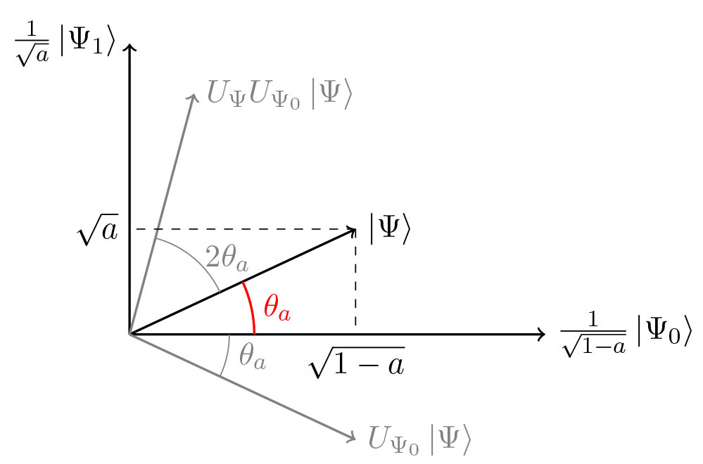
- We can rewrite $Q = U_\Psi U_{\Psi_0}$, where $U_\Psi = 2 \ket{\Psi}\bra{\Psi} - I$ and $U_{\Psi_0} = \frac{2}{1-a} \ket{\Psi_0}\bra{\Psi_0} - I$.
Matrix representation of $Q$
\[\begin{split} Q \ket{\Psi_1} & = U_\Psi U_{\Psi_0} \ket{\Psi_1} = - U_\Psi \ket{\Psi_1} = (I - 2 \ket{\Psi}\bra{\Psi}) \ket{\Psi_1} \\ & = \ket{\Psi_1} - 2a\ket{\Psi} = (1-2a)\ket{\Psi_1}-2a\ket{\Psi_0} \\ Q \ket{\Psi_0} & = U_\Psi \ket{\Psi_0} = (2 \ket{\Psi}\bra{\Psi} - I) \ket{\Psi_0} \\ & = 2(1-a) \ket{\Psi} - \ket{\Psi_0} = 2(1-a) \ket{\Psi_1} + (1-2a) \ket{\Psi_0} \end{split}\]Using $\sin^2(\theta_a) = a$ and $\cos^2(\theta_a) = 1-a$, we get:
\[\begin{split} Q \frac{\ket{\Psi_1}}{\sqrt{a}} & = (1-2a) \frac{\ket{\Psi_1}}{\sqrt{a}} - 2\sqrt{a(1-a)} \frac{\ket{\Psi_0}}{\sqrt{1-a}} \\ &= (1-2\sin^2(\theta_a)) \frac{\ket{\Psi_1}}{\sqrt{a}} - 2\cos(\theta_a)\sin(\theta_a) \frac{\ket{\Psi_0}}{\sqrt{1-a}} \\ &= \cos(2\theta_a) \frac{\ket{\Psi_1}}{\sqrt{a}} - \sin(2\theta_a) \frac{\ket{\Psi_0}}{\sqrt{1-a}} \\ Q \frac{\ket{\Psi_0}}{\sqrt{1-a}} & = \sin(2\theta_a) \frac{\ket{\Psi_1}}{\sqrt{a}} + \cos(2\theta_a) \frac{\ket{\Psi_0}}{\sqrt{1-a}} \end{split}\]- Thus, $Q$ is a rotation matrix in the basis ${\frac{1}{\sqrt{a}} \ket{\Psi_1}, \frac{1}{\sqrt{1-a}} \ket{\Psi_0}}$:
-
It has eigenvalues $e^{2i\theta_a}, e^{-2i\theta_a}$ with corresponding eigenvectors $\frac{1}{2} \begin{pmatrix} 1 \ i \end{pmatrix}, \frac{1}{2} \begin{pmatrix} 1 \ -i \end{pmatrix}$, noted $\ket{\Psi_+}$ and $\ket{\Psi_-}$.
-
We can now write $\ket{\Psi}$ in the $Q$-eigenvector basis:
\(\ket{\Psi} = \frac{-i}{2} (e^{i\theta_a} \ket{\Psi_+} - e^{-i\theta_a} \ket{\Psi_-})\) and it follows that:
\[Q^j \ket{\Psi} = \frac{-i}{2} (e^{(2j+1)i\theta_a} \ket{\Psi_+} - e^{-(2j+1)i\theta_a} \ket{\Psi_-})\]- By writing it back in the original ${\frac{1}{\sqrt{a}} \ket{\Psi_1}, \frac{1}{\sqrt{1-a}} \ket{\Psi_0}}$ basis:
-
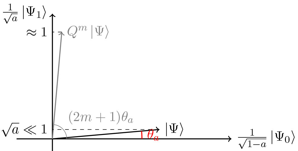
After $m$ applications of the operator $Q$, measuring the state $\ket{\Psi}$ produces a good state with probability equal to $\sin^2((2m+1) \theta_a)$.
-
$x \mapsto \sin^2((2x+1) \theta_a)$ is maximized for $x = \frac{\pi}{4 \theta} - \frac{1}{2}$.
-
Thus the probability is maximized for $m = \left \lfloor{\pi/(4\theta_a)}\right \rfloor $ (when the value of $a$ is known).
-
We can show that $\sin^2((2m+1) \theta_a) \geq 1-a$.
Complexity of the algorithm
-
We use $2m+1$ applications of $\mathcal{A}$ and $\mathcal{A}^\dagger$.
-
Since $\theta_a \approx \sin(\theta_a) = \sqrt{a}$, we get:
- And the success probability is $1-a \approx 1$.
Visual demo
And indeed $m = \left \lfloor{\pi/4\theta_a}\right \rfloor = 11$.
Grover’s algorithm
$\ket{\Psi} = \frac{1}{\sqrt{N}} \sum_{x = 0}^{N-1} \ket{x}$ and $\chi = \mathbb{1}_{x = 0}$. Then $a = 1/N \ll 1$, \(m = \left \lfloor{\frac{\pi}{4\theta_a}}\right \rfloor \approx \left \lfloor{\frac{\pi}{4 \sin \theta_a}}\right \rfloor = \left \lfloor{\frac{\pi \sqrt{N}}{4}}\right \rfloor = \mathcal{O}(\sqrt{N})\) and we get the state $\ket{0}$ with probability $\sin^2((2m+1) \theta_a) \geq 1-a \approx 1$.
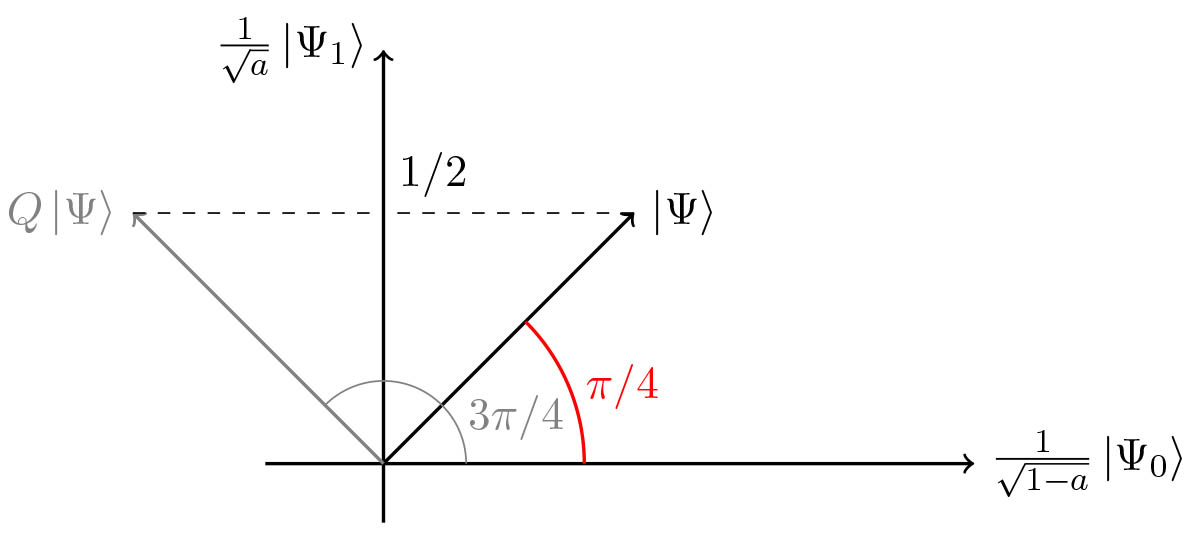
A special case
$\ket{\Psi} = \frac{1}{\sqrt{2}} (\ket{0} + \ket{1}) \ket{x}$ and $\chi = \mathbb{1}_{x = 0}$. We have $a = 1/2$, $\theta_a = \frac{\pi}{4}$. Then, $m = 1$ and $\sin^2((2m+1) \theta_a) = \sin^2 \frac{3\pi}{4} = \frac{1}{2} = a$. Amplitude amplification has no effect.
Amplitude amplification when $a$ is not known
- When $a$ is not known, we can first estimate it using quantum amplitude estimation (see next section) and then run the previous algorithm by replacing the exact $a$ by its estimate.
-
Another approach is to use QSearch. The intuition is the following: \(\text{for } \theta \sim \mathcal{U}[0, 2\pi], \E \left[\sin^2 \theta\right] = \frac{1}{2}\) By choosing $M$ sufficiently large, $M \theta_a$ is large and by picking $j \in_U [1, M]$, $j \theta_a \text{ mod } 2\pi$ follows a good approximation of $\mathcal{U}[0, 2\pi]$ (and so does $(2j+1) \theta_a \text{ mod } 2\pi$).
-
Then, the probability $\sin^2((2j+1)\theta_a)$ that the measurement produces a good state is in average $\frac{1}{2}$.
- Since we don’t know $\theta_a$, we use an exponential search space for $M = c^l$ by iteratively incrementing the value of $l$ for a constant $c$.
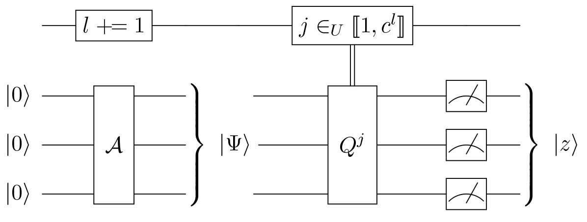
The QSearch algorithm
Initialization: $l = 0$.
Repeat: (while $\ket{z}$ is not a good state)
Quantum de-randomization when $a$ is known
The success probability of the Quantum Amplitude Amplification algorithm is $1-a$. It turns out we can actually find a good solution with certainty.
-
$m \mapsto \sin^2((2m+1) \theta_a)$ is maximized for $\tilde{m} = \frac{\pi}{4 \theta} - \frac{1}{2}$.
-
If $\tilde{m}$ is an integer, $\sin^2((2\tilde{m}+1) \theta_a) = 1$.
-
Else we use $m = \left \lceil{\tilde{m}}\right \rceil = \left \lfloor{\pi/(4\theta_a)}\right \rfloor$ iterations, which is slightly too much.
The de-randomization approach is the following:
- Apply $Q$ only $\left \lfloor{\tilde{m}}\right \rfloor$ times. The resulting state is:
- We further define $Q’(\phi, \varphi) = - \mathcal{A} S_0(\phi) \mathcal{A}^\dagger S_\chi(\varphi)$
-
$Q = Q’(\phi = \pi, \varphi = \pi)$
-
By applying one final $Q’(\phi, \varphi)$, we obtain:
- We can choose $\phi$ and $\varphi$ so that the coefficient in front of $\ket{\Psi_0}$ = 0: \(\begin{split} \iff \cot((2\left\lfloor{\tilde{m}}\right\rfloor+1)\theta_a) & = e^{i\varphi} 2\sqrt{a(1-a)} \frac{1-e^{i\phi}}{2((1-e^{i\phi})a+e^{i\phi})} \\ &= e^{i\varphi} \sin(2\theta_a) (2\underbrace{a}_{= 1-\cos(2\theta_a)} + \frac{2e^{i\phi}}{1-e^{i\phi}})^{-1} \\ &= e^{i\varphi} \sin(2\theta_a) (-\cos(2\theta_a) + \underbrace{\frac{1+e^{i\phi}}{1-e^{i\phi}}}_{= i\cot(\phi/2)})^{-1} \end{split}\)
III. Quantum amplitude estimation
-
Amplitude amplification: find $x \in X$ such that $\chi(x) = 1$.
-
Amplitude estimation: estimate $a = \bra{\Psi_1}\ket{\Psi_1}$.
-
By $a = \sin^2(\theta_a)$, an estimate for $a$ translates into an estimate for $\theta_a$.
-
The eigenvalues of $Q$ are $\lambda_+ = e^{2i\theta_a}$ and $\lambda_- = e^{-2i\theta_a}$, so we can instead estimate one of these eigenvalues.
-
Let us define the operator
so that e.g:
\[\Lambda_M(Q) \ket{j}\ket{\Psi_+} = e^{2i\theta_aj}\ket{j}\ket{\Psi_+}\]- We recall the quantum Fourier transform (for $x \in {0, \dots, M-1}$):
- And we define (for a real $0 \leq \omega < 1$):
\(\ket{S_M(\omega)} = \frac{1}{\sqrt{M}} \sum_{y=0}^{M-1} e^{2\pi i\omega y} \ket{y}\) so that, for $x \in {0, \dots, M-1}$: $\ket{S_M(x/M)} = F_M \ket{x}$.
Quantum circuit for amplitude estimation
$(F_M^{-1} \tens I)(\Lambda_M(Q))(F_M \tens I)$ applied on the state $\ket{0} \tens \mathcal{A} \ket{0}$
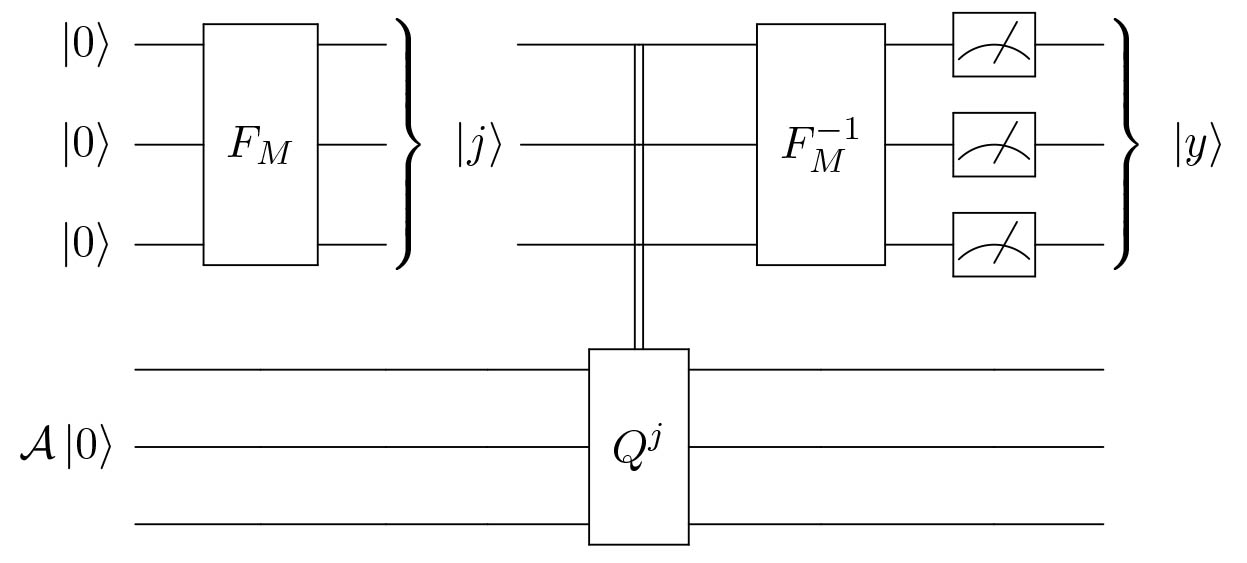
(If $M$ is a power of 2, we can replace the Quantum Fourier transforms by Hadamard gates)
Proof of correctness
The quantum circuit corresponds to the unitary transformation $(F_M^{-1} \tens I)(\Lambda_M(Q))(F_M \tens I)$ applied on the state $\ket{0} \tens \mathcal{A} \ket{0}$, with
\[\mathcal{A} \ket{0} = -\frac{i}{\sqrt{2}}(e^{i \theta_a} \ket{\Psi_+} - e^{-i \theta_a} \ket{\Psi_-})\]By applying $F_M \tens I$:
\[\frac{1}{\sqrt{2M}}\sum_{j=0}^{M-1} \ket{j} \tens (e^{i \theta_a} \ket{\Psi_+} - e^{-i \theta_a} \ket{\Psi_-})\]After applying $\Lambda_M(Q)$:
\[\frac{e^{i \theta_a}}{\sqrt{2}} \ket{S_M(\theta_a/\pi)} \tens \ket{\Psi_+} - \frac{e^{-i \theta_a}}{\sqrt{2}} \ket{S_M(1 - \theta_a/\pi)} \tens \ket{\Psi_-}\]- Finally, after $F_M^{-1} \tens I$, we have:
-
By tracing out the second register in the eigenvector basis ${\ket{\Psi_+}, \ket{\Psi_-}}$, we obtain a $\frac{1}{2}$-$\frac{1}{2}$ mixture of $F_M^{-1} \ket{S_M(\theta_a/\pi)}$ and $F_M^{-1} \ket{S_M(1 - \theta_a/\pi)}$.
-
By symmetry (since $\sin^2(\pi \frac{y}{M}) = \sin^2(\pi (1 - \frac{y}{M}))$), we can assume the measured $\ket{y}$ is the result of measuring $F_M^{-1} \ket{S_M(\theta_a/\pi)}$.
-
We thus have $\tilde{\theta_a} = \pi \frac{y}{M}$ is a good estimate of $\theta_a$ (see next slide).
Bounding the error of the estimate
$\frac{1}{M} F_M^{-1} \ket{S_M(\omega)}$ is a good estimate of $\omega$. Indeed, if $\omega = x/M$ for some $0 \leq x < M$, then $F_M^{-1} \ket{S_M(x/M)} = \ket{x}$. Otherwise:
Theorem:
Let $X$ be the r.v. corresponding to the result of measuring $F_M^{-1} \ket{S_M(\omega)}$. Then:
\[\mathbb{P}\left(\left|\frac{1}{M} X - \omega \right| \leq \frac{1}{M}\right) \geq \frac{8}{\pi^2} \approx 0.81\]Lemma:
Letting $\Delta = \left|\frac{1}{M} x - \omega \right|$ for some $x \in {0, \dots, M-1}$, we have:
\[\mathbb{P}[X = x] = \frac{\sin^2(M\Delta\pi)}{M^2\sin^2(\Delta\pi)}\]Proof of the Lemma:
\[\begin{split} \mathbb{P}[X = x] &= |\bra{x}F_M^{-1}\ket{S_M(\omega)}|^2 \\ &= |(F_M \ket{x})^\dagger \ket{S_M(\omega)}|^2 \\ &= |\braket{S_M(x/M)}{S_M(\omega)}|^2 \\ &= \left|(\frac{1}{\sqrt{M}} \sum_{y=0}^{M-1} e^{2\pi i x/M y} \bra{y})(\frac{1}{\sqrt{M}} \sum_{y=0}^{M-1} e^{2\pi i \omega y} \ket{y}) \right|^2 \\ &= \frac{1}{M^2} \left|\sum_{y=0}^{M-1}e^{2\pi i \Delta y} \right|^2 = \frac{\sin^2(M\Delta\pi)}{M^2\sin^2(\Delta\pi)} \end{split}\]Proof of the Theorem:
\[\begin{split} \mathbb{P}[d(X/M, \omega) \leq 1/M] & = \mathbb{P}[X = \left\lfloor{M\omega}\right\rfloor] + \mathbb{P}[X = \left\lceil{M\omega}\right\rceil] \\ & = \frac{\sin^2(M\Delta\pi)}{M^2\sin^2(\Delta\pi)} + \frac{\sin^2(M(\frac{1}{M} - \Delta)\pi)}{M^2\sin^2((\frac{1}{M} - \Delta)\pi)} \\ & \geq \frac{8}{\pi^2} \end{split}\]Since the minimum of this expression is reached at $\Delta = 1/(2M)$.
A bounding error on $\tilde{\theta_a}$ translates into a bound on $\tilde{a}$.
Lemma:
Let $a = \sin^2(\theta_a)$ and $\tilde{a} = \sin^2(\tilde{\theta_a})$ with $0 \leq \theta_a, \tilde{\theta_a} \leq \frac{\pi}{2}$. Then:
\[|\tilde{\theta_a} - \theta_a| \leq \epsilon \Longrightarrow |\tilde{a} - a| \leq 2 \epsilon \sqrt{a (1-a)} + \epsilon^2\]A bounding error on $\tilde{\theta_a}$ translates into a bound on $\tilde{a}$.
Proof:
\[\begin{split} \tilde{a} - a & = \sin^2(\tilde{\theta_a}) - \sin^2(\theta_a) \leq \sin^2(\theta_a + \epsilon) - \sin^2(\theta_a) \\ & = (\sin(\theta_a)\cos(\epsilon) + \sin(\epsilon)\cos(\theta_a))^2 - \sin^2(\theta_a) \\ &= \sin^2(\theta_a)\cos(\epsilon)+\sin^2(\epsilon)\cos^2(\theta_a)+2\cos(\theta_a)\sin(\theta_a)\cos(\epsilon)\sin(\epsilon) \\ & ~~~ -\sin^2(\theta_a) \\ &= \sin^2(\epsilon) (\cos^2(\theta_a) - \sin^2(\theta_a)) + \sqrt{a(1-a)}\sin^2(\epsilon)\\ & = \sqrt{a(1-a)}\sin(2\epsilon)+(1-2a)\sin^2(\epsilon) \\ & \leq 2 \epsilon \sqrt{a(1-a)} + \epsilon^2 \end{split}\]Same for $a - \tilde{a}$.
Combining those results, the Amplitude Estimation algorithm outputs $\tilde{\theta_a}$ such that
\[|\tilde{\theta_a}/\pi - \theta_a/\pi| \leq \frac{1}{M}\] \[\iff |\tilde{\theta_a} - \theta_a| \leq \frac{\pi}{M}\]with probability greater than $8/\pi^2$.
Thus, by setting $\epsilon = \frac{\pi}{M}$:
\[|\tilde{a} - a| \leq 2 \pi \frac{\sqrt{a(1-a)}}{M} + \frac{\pi^2}{M^2}\]Applications
1. Application to counting
The amplitude estimation algorithm can be used for counting the number of good elements $t = \left|{x \in X \text{ s.t. } \chi(x) = 1}\right|$
- By choosing $\mathcal{A} = F_N$ the Quantum Fourier Transform:
- we have:
Thus, $a = \bra{\Psi_1}\ket{\Psi_1} = \frac{1}{N}$, and so $t = a \times N$.
2. Application to Monte Carlo sampling
-
Let $X$ be a random variable taking values ${0, \dots, N}$ with probability $p_i$. We want to compute $\mathbb{E}[f(X)]$.
-
Using Monte Carlo sampling, with $M$ evaluations of $f$, we get: \(\frac{1}{M} \sum_{k=0}^M f(X_k) \approx \mathbb{E}[f(X)] \pm \frac{C}{\sqrt{M}}\)
-
Quantum approach: define
and the operator
\[F: \ket{i} \tens \ket{0} \mapsto \ket{i} \tens (\sqrt{1 - f(i)} \ket{0} + \sqrt{f(i)} \ket{1})\]Then:
\[F \ket{\Psi} \tens \ket{0} = \sum_{i=0}^{N-1} \sqrt{1-f(i)}\sqrt{p_i} \ket{i} \tens \ket{0} + \sqrt{f(i)} \sqrt{p_i} \ket{i} \tens \ket{1}\]Using amplitude estimation, we estimate the probability to measure $\ket{1}$ in the last Qbit: $\tilde{a} = \sum_{i=0}^{N-1} p_i f(i) = \mathbb{E}[f(X)]$, and using $M$ evaluations of $f$:
\[\left|\tilde{a} - a\right| \leq 2\pi\frac{\sqrt{a(a-a)}}{M} + \frac{\pi^2}{M^2}\]with a convergence rate of $\mathcal{O}(\frac{1}{M})$ to be compared to the classical $\mathcal{O}(\frac{1}{\sqrt{M}})$ rate.
3. Application to Quantum Risk Analysis
-
Quantum Risk Analysis (IBM Research - Zurich): In quantitative finance, VaR (Value at Risk) and CVaR (Conditional Value at Risk) are typically estimated using Monte Carlo sampling of the relevant probability distribution.
-
For a confidence value $\alpha \in [0, 1]$, $\text{VaR}_\alpha(X)$ is the smallest $l$ such that $\mathbb{P}[X \leq l] \geq (1-\alpha)$.
-
By defining $f_l(x) = 1$ if $\mathbb{1}_{x \leq l}$, we thus want to approximate $\mathbb{P}[X \leq l] = \mathbb{E}[f_l(X)]$ of a random variable $X$ taking values ${0, \dots, N}$ with probability $p_i$.
IV. Conclusion
- Quadratic speedup: this speedup is in fact the best we can attain.
- Even if amplitude amplification and estimation doesn’t solve NP-complete problems in polynomial time, we can apply it to more than just search problems, such as Monte Carlo sampling with a non-negligible speedup.