U-Net for Road Segmentation
Report: unet.pdf
GitHub: UNet
In this project we implement an encoder-decoder convolutional neural network to segment roads in a dataset of aerial images, resulting in significant improvement compared to logistic regression and patch-wise CNN, and reaching an F score of 0.94.
I - Introduction
In this project, we are training a classifier to segment roads in aerial images from Google Maps, given the ground-truth images, i.e. the pixel-level labeled images ($1$ corresponding to a road, $0$ to background).
The train dataset contains 100 labeled images of $400 \times 400$ pixels. After the training, we run a prediction on $50$ test images of $608 \times 608$ pixels. The predicted images are then cropped in patches of $16 \times 16$ pixels and transformed to a csv submission file containing the predicted output ($1$ for a road, $0$ for background) for each patch.
This report is structured as follows. Section II describes the architecture of our encoder-decoder CNN model. Section III details the procedure we use to further refine the predictions of the model. We include the experimental settings, baselines, and final results in Section IV. Section V concludes the report.
II - Encoder-Decoder CNN
Here we present an encoder-decoder convolutional neural network architecture that is similar to the models proposed in [7], [1]. The network consists of two parts, a convolutional network and a deconvolutional network. The figure below gives an illustration of our model. The convolutional network extracts high-level features from the input image, and the deconvolutional network builds a segmentation based on the extracted features. The output of the whole encoder-decoder network is then a probability map with the same size as the input image, which indicates the probability of each pixel belonging to a road.
In order to down-sample the layers by a factor of $2$ once in a while, we use a convolutional layer with stride $2$ instead of a max pooling layer. Similarly, we use a deconvolutional layer with stride $2$ to up-sample the layers by a factor of $2$, allowing us to reconstruct the size of the original image.
However, the predictions of the decoder part of the model can be rather coarse. Intuitively, we want to combine those predictions with fine details from the low-level layers. To do this, we fuse information from previous layers to specific layers in the deconvolutional network [5], as indicated by the directed lines in the next figure.

The specifications of our model are detailed in the next table. We use ReLU as the activation function. We use a padding scheme such that the output size is $\lceil\textrm{input size}/\textrm{stride}\rceil$.
| Layer | Kernel size | Stride | Output size |
|---|---|---|---|
input |
$-$ | $-$ | $320\times 320\times 3$ |
conv_1_1 |
$3\times 3$ | $1$ | $320\times 320\times 64$ |
conv_1_2 |
$3\times 3$ | $2$ | $160\times 160\times 64$ |
conv_2_1 |
$3\times 3$ | $1$ | $160\times 160\times 128$ |
conv_2_2 |
$3\times 3$ | $2$ | $80\times 80\times 128$ |
conv_3_1 |
$3\times 3$ | $1$ | $80\times 80\times 256$ |
conv_3_2 |
$3\times 3$ | $1$ | $80\times 80\times 256$ |
conv_3_3 |
$3\times 3$ | $2$ | $40\times 40\times 256$ |
conv_4_1 |
$3\times 3$ | $1$ | $40\times 40\times 512$ |
conv_4_2 |
$3\times 3$ | $1$ | $40\times 40\times 512$ |
conv_4_3 |
$3\times 3$ | $2$ | $20\times 20\times 512$ |
conv_5_1 |
$3\times 3$ | $1$ | $20\times 20\times 512$ |
conv_5_2 |
$3\times 3$ | $1$ | $20\times 20\times 512$ |
conv_5_3 |
$3\times 3$ | $2$ | $10\times 10\times 512$ |
conv_6_1 |
$3\times 3$ | $1$ | $10\times 10\times 512$ |
conv_6_2 |
$3\times 3$ | $1$ | $10\times 10\times 512$ |
conv_6_3 |
$3\times 3$ | $2$ | $5\times 5\times 512$ |
deconv_6_3 |
$3\times 3$ | $2$ | $10\times 10\times 512$ |
deconv_6_2 |
$3\times 3$ | $1$ | $10\times 10\times 512$ |
deconv_6_1 |
$3\times 3$ | $1$ | $10\times 10\times 512$ |
deconv_5_3 |
$3\times 3$ | $2$ | $20\times 20\times 512$ |
deconv_5_2 |
$3\times 3$ | $1$ | $20\times 20\times 512$ |
deconv_5_1 |
$3\times 3$ | $1$ | $20\times 20\times 512$ |
deconv_4_3 |
$3\times 3$ | $2$ | $40\times 40\times 512$ |
deconv_4_2 |
$3\times 3$ | $1$ | $40\times 40\times 512$ |
deconv_4_1 |
$3\times 3$ | $1$ | $40\times 40\times 256$ |
deconv_3_3 |
$3\times 3$ | $2$ | $80\times 80\times 256$ |
deconv_3_2 |
$3\times 3$ | $1$ | $80\times 80\times 256$ |
deconv_3_1 |
$3\times 3$ | $1$ | $80\times 80\times 128$ |
deconv_2_2 |
$3\times 3$ | $2$ | $160\times 160\times 128$ |
deconv_2_1 |
$3\times 3$ | $1$ | $160\times 160\times 64$ |
deconv_1_2 |
$3\times 3$ | $2$ | $320\times 320\times 64$ |
deconv_1_1 |
$3\times 3$ | $1$ | $320\times 320\times 64$ |
output |
$1\times 1$ | $1$ | $320\times 320\times 2$ |
III - Post-Processing
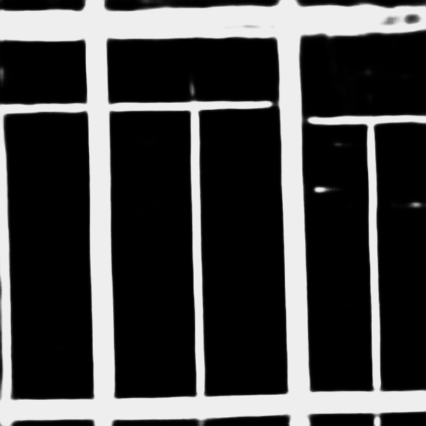
With our current encoder-decoder CNN model, the predictions may have discontinuity points or holes in the roads, as the next figure shows.
To address this problem, we adopt a post-processing procedure [6] which enables to refine the predictions given by the encoder-decoder CNN. Let $f$ be the network trained to output the predictions of the input images $X$, which we denote by $Y_p$. We build another network $f_p$ that takes the same functional form as $f$, and train it using $Y_p$ as input and the groundtruth images as labels. The output of $f_p$ is then used as our final predictions.
IV - Evaluation
In this section, we elaborate on the experiment settings, including how we augment the data and train the model. We then evaluate the performance of our model as well as the baselines, followed by some analysis and discussion.
A. Data Augmentation
The original training dataset contains $100$ aerial images. For each of these images, we apply a rotation of $45$, $90$, $-45$, $-90$ degrees respectively, which aims to increase the number of examples with diagonal roads in the dataset, and crop out the central part to obtain four new aerial images of size $320\times 320$. Besides, for this original image, we also crop out a region of size $320\times 320$ at each of the four corners. Again, we rescale the original image to $320\times 320$ to get another new image. Thus, for each training image, we can generate nine new images, resulting in an augmented dataset of $900$ aerial images. We then split our augmented data into a training set ($90$%, i.e. $810$ images) and a testing set ($10$%, i.e. $90$ images).
B. Baselines
For the baselines, the problem is framed as a binary classification task. We extract patches of $k \times k$ pixels from the training images. For each patch, the label can be obtained by looking at the corresponding groundtruth image, and we can perform a binary classification to determine if it corresponds to a road or to background. The hyper-parameter $k$ is crucial since it should optimize the following trade-off: a larger $k$ means that our prediction will be more accurate since the model has more information from the pixels to make its prediction; a smaller $k$ enables a more fine-grained grid of patches.
Logistic Regression: For each patch, we compute the mean and variance values for each of the three channels, thus obtaining a feature vector with size $6$. We then train a simple logistic regression model on the feature vectors.
Naïve CNN: We train a naïve convolutional neural network directly on the patches. The specifications of the network are detailed in the next table. Note that the input size, depending on the value of patch size $k$, is not fixed at $16\times 16$.
| Layer | Kernel size | Stride | Output size |
|---|---|---|---|
input |
$-$ | $-$ | $16\times 16\times 3$ |
conv_1 |
$5\times 5$ | $1$ | $16\times 16\times 32$ |
pool_1 |
$2\times 2$ | $2$ | $8\times 8\times 32$ |
conv_2 |
$5\times 5$ | $1$ | $8\times 8\times 64$ |
pool_2 |
$2\times 2$ | $2$ | $4\times 4\times 64$ |
fc_3 |
$4\times 4$ | $-$ | $1\times 1\times 512$ |
output |
$1\times 1$ | $-$ | $1\times 1\times 2$ |
C. Training
Logistic Regression: We train the logistic regression using an inverse regularization strength of $10^5$, Liblinear solver and a balanced class-weight (so that classes with a lower number of occurrences are fitted equally).
Naïve CNN: We train the CNN with 50 epochs, an initial learning rate of $0.01$ (that decays exponentially), simple momentum for the optimization and a regularization coefficient of $5 \times 10^{-4}$. For this model, the patch-size must be both a divisor of the size of the image and a multiple of 4 (since the input image is pooled twice during the forward pass).
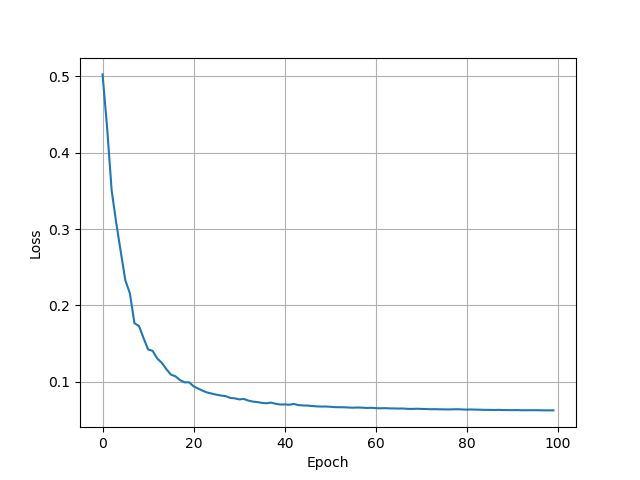
Encoder-decoder CNN: We apply batch normalization [4] to each of the convolutional and deconvolutional layers, to alleviate the problem of internal covariate shift. We add three drop out layers [3] with keep probability $0.5$ to the network, after deconv_4_1, deconv_3_1, and deconv_2_1, respectively. To train the model, we use stochastic gradient descent with learning rate of $5.0$ and batch size of $5$. The network is trained for $100$ epochs on the training images, and $10$ epochs for the post-processing procedure. It roughly takes three hours to finish the whole training procedure on an NVIDIA GTX 1080 graphics card. The next figure shows the evolution of the cross-entropy loss during the training procedure. We can observe that after $40$ epochs, the loss ($0.070346$) is almost the same as the final loss ($0.06267$).
D. Results
To evaluate the models, the predicted images are cropped into patches of $16 \times 16$ pixels, in order to compare scores on a same basis.
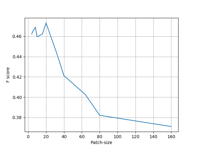
First of all, to see the impact of the patch size on the performance of the baselines, we train a logistic regression model using several patch sizes. The result is shown in the next figure. In particular, we get better results with a patch size of $8$ or $20$ in the case of logistic regression. Therefore, in addition to a patch size of $16$, we also include models with patch size $8$ and $20$ in the final comparison.
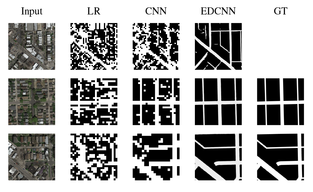
We train each model on the training set ($90$% of the augmented data) and compute the accuracy, precision, recall and F score on the validation set ($10$% of the data), which are listed in the next table. As the training of our encoder-decoder CNN model is long, we compute the score only once. In particular, we do not adopt a cross-validation procedure to get this score and we thus have no information about its variability. The logistic regression and naïve CNN models with patch size $k$ are denoted by LR$k$ and CNN$k$ respectively. EDCNN is our encoder-decoder CNN model. We can see that our model outperforms both of the two baselines. A comparison of the predictions given by all the models are shown in the previous figure.
| Model | Accuracy | Precision | Recall | F score |
|---|---|---|---|---|
| LR16 | 0.5919 | 0.3442 | 0.6859 | 0.4585 |
| LR8 | 0.5522 | 0.3348 | 0.7888 | 0.4701 |
| LR20 | 0.5589 | 0.3394 | 0.7940 | 0.4755 |
| CNN8 | 0.7874 | 0.5463 | 0.9186 | 0.6852 |
| CNN20 | 0.8126 | 0.5854 | 0.8772 | 0.7022 |
| CNN16 | 0.8598 | 0.6703 | 0.8726 | 0.7583 |
| EDCNN | 0.9654 | 0.9469 | 0.9345 | 0.9406 |
To get a general sense of the various features extracted by the encoder-decoder CNN, we give an illustration of the intermediate layers (both convolutional and deconvolutional) in the next figure.

V - Conclusion
In this project, we implement an encoder-decoder model that we train and test on aerial images, obtaining an F score of 0.94 and observing significant improvements compared to simples baselines. Further improvements including atrous convolutions or pyramid pooling modules could be added to our encoder-decoder structure to reach state of the art performance (e.g. DeepLab v3 [2]) but seem out of reach in the context of this course.
References
[1] V. Badrinarayanan, A. Handa, and R. Cipolla. Segnet: A deep convolutional encoder-decoder architecture for robust semantic pixel-wise labelling. arXiv preprint arXiv:1505.07293, 2015.
[2] L.-C. Chen, G. Papandreou, F. Schroff, and H. Adam. Rethinking atrous convolution for semantic image segmentation. arXiv preprint arXiv:1706.05587, 2017.
[3] G. E. Hinton, N. Srivastava, A. Krizhevsky, I. Sutskever, and R. R. Salakhutdinov. Improving neural networks by preventing co-adaptation of feature detectors. arXiv preprint arXiv:1207.0580, 2012.
[4] S. Ioffe and C. Szegedy. Batch normalization: Accelerating deep network training by reducing internal covariate shift. In International Conference on Machine Learning, pages 448–456, 2015.
[5] J. Long, E. Shelhamer, and T. Darrell. Fully convolutional networks for semantic segmentation. In Proceedings of the IEEE Conference on Computer Vision and Pattern Recognition, pages 3431–3440, 2015.
[6] V. Mnih and G. E. Hinton. Learning to detect roads in high-resolution aerial images. In European Conference on Computer Vision, pages 210–223. Springer, 2010.
[7] H. Noh, S. Hong, and B. Han. Learning deconvolution network for semantic segmentation. In Proceedings of the IEEE International Conference on Computer Vision, pages 1520–1528, 2015.